Overview
The objective of this text is to describe qualitatively the general framework developed in the Structural Mechanics Application related to the “Constitutive Law” problem in engineering. The main point of focus is the description of various constitutive models based on phenomenological hyperelasticity, elastoplasticity, damage, viscoelasticity and elasto-viscoplasticity.
Since this is a work-in-progress, we are going to describe the present state of the Application but some other constitutive models will be added in the future. This is why we encourage you to propose new methodologies to be implemented. We are always willing to develop some useful tools for other engineers and professionals.
At this point, there are some Constitutive Laws (CL from now on) that are available and ready to use:
- Overview
- Isotropic Elasticity
- HyperElasticity
- Isotropic Plasticity
- Small Strain Isotropic Damage
- Small Strain d+d- Damage
- ViscoElasticity
- ViscoPlasticity
- Appendix
- References
- Contact us!
A description of the previous models will be done in the following paragraphs.
Isotropic Elasticity
This is the most simple CL but also one of the most used. Isotropic materials require two material parameters only, the Young modulus E and the Poisson’s ratio v. The constitutive matrix for isotropic materials can be directly written in global cartesian axes. If initial strains and stresses are taken into account we can write:
σ=D : ε
being ε the strain tensor assuming small strains and D the Elastic Isotropic Constitutive Matrix expressed as:
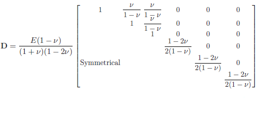 The procedure is analogous with the 2D and axisymmetric case.
HyperElasticity
Common properties
It can be shown that the stored strain energy (potential) for a hyperelastic material which is isotropic with respect to the initial, unstressed configuration can be written as a function of the principal invariants (I1, I2, I3) of the right Cauchy–Green deformation tensor. The principal invariants of a second-order tensor and their derivatives figure prominently in elastic and elastic–plastic constitutive relations. [5]
Kirchhoff Material
Many engineering applications involve small strains and large rotations. In these problems the effects of large deformation are primarily due to rotations (such as in the bending of a marineriser or a fishing rod). The response of the material may then be modeled by a simple extension of the linear elastic laws by replacing the stress by the PK2 stress and the linear strain by the Green strain. This is called a Saint Venant–Kirchhoff material, or a Kirchhoff material for brevity. The most general Kirchhoff model is:
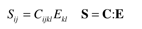
The definition of the of the constitutive tensor for the Kirchoff model is:

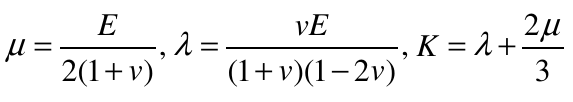
The two independent material constants l and m are called the Lamé constants. The stress–strain relation for an isotropic Kirchhoff material may therefore be written as:

The Lamé constants can be expressed in terms of other constants which are more closely related to physical measurements, the bulk modulus K, Young’s modulus E and Poisson’s ratio v, by:
Neo-Hookean Material
The Neo-Hookean material model is an extension of the isotropic linear law (Hooke’s law) to large deformations. The stored energy function for a compressible Neo-Hookean material (isotropic with respect to the initial, unstressed configuration) is:
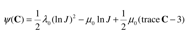
The stresses are given by:
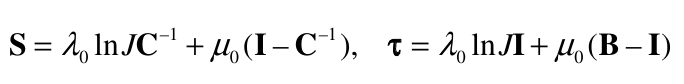
The elasticity tensors:
Isotropic Plasticity
Brief summary of the modular design
Introduction
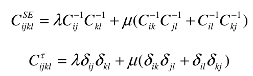
In order to understand the structure of the plasticity CL one can see the methodology as a set of Matryoshka dolls as shown in the following picture:
In which each object is “templated” inside the bigger one. In this sense the registration of the Plasticity Laws follows the same idea:
GenericSmallStrainIsotropicPlasticity<GenericConstitutiveLawIntegratorPlasticity<VonMisesYieldSurface<ModifiedMohrCoulombPlasticPotential<6>>>>
In this case we have registered a Plasticity CL using the Von Mises YS and a Modified Mohr Coulomb PP.
Yield Surface
This object is used to determine whether the strain/stress tensor is in elastic or plastice regime. There are several classical yield surfaces available right now:
- Rankine
- Tresca
- Von Mises (J2)
- Modified Mohr Coulomb (see appendix)
- Drucker-Prager
- Simo-Ju
- Classical Mohr-Coulomb
The general definition of the yield surface class is as follows:
template<class TPlasticPotentialType>
class KRATOS_API(STRUCTURAL_MECHANICS_APPLICATION) DruckerPragerYieldSurface
As explained before, the Plasticity constitutive Law could use one yield surface and a different plastic potential surface (so-called non-associative plasticity) so we had to develop a strategy to allow different YS-PP combinations without repeating code. This was done again, by including the PP as a template for the Yield Surface.
Plastic Potential
This object is used to compute the derivatives of the Plastic potential surfaces in order to calculate the direction of the plastic strain. The general definition of the PP is:
template <SizeType TVoigtSize = 6>
class KRATOS_API(STRUCTURAL_MECHANICS_APPLICATION) DruckerPragerPlasticPotential
There are several classical plastic potential surfaces available:
- Tresca
- Von Mises (J2)
- Modified Mohr-Coulomb (see appendix)
- Drucker-Prager
- Classical Mohr-Coulomb
It is important to mention that the Tresca, Modified Mohr-Coulomb and the classical Mohr-Coulomb have been smoothed when the stress state is close to the edges of the yield surface. In the case of Tresca the surface is smoothed with Von-Mises whereas in the case of Mohr-Coulomb is smoothed with Drucker-Prager.
Flow Rules
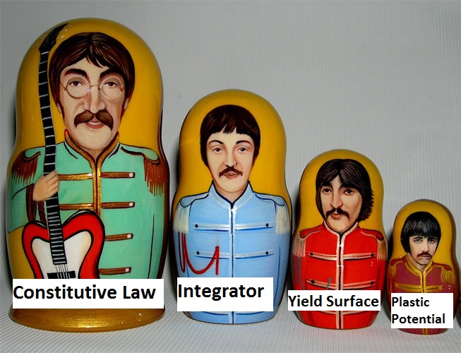
We have implemented a plasticity algorithm that allows the following evolution laws of the yield surface:
- Linear Softening
- Exponential Softening
- Hardening + Softening
- Perfect Plasticity
- Curve fitting hardening
The previous curves can be seen in the following graph:
Small Strain Plasticity
General Description
The theory of plasticity is concerned with solids that, after being subjected to a loading programme, may sustain permanent (or plastic) deformations when completely unloaded. In particular, this theory is restricted to the description of materials (and conditions) for which the permanent deformations do not depend on the rate of application of loads and is often referred to as rate-independent plasticity.
It is important to remark that the model presented here is restricted to infinitesimal deformations but some large strain models are going to be implemented in the future. As usual, this constitutive law requires a Yield Surface (YS) in order to detect de non-linear behaviour and a Plastic Potential (PP) to describe the direction of the plastic strain.
Since there are several options to be used for YS and PP and taking into account that they can be combined in any way, we have developed a method of assembling them as required, automatically, by using a factory procedure.
The more general file is called generic_small_strain_isotropic_plasticity.cpp and the main method is CalculateMaterialResponseCauchy as follows:
template <class TConstLawIntegratorType>
void GenericSmallStrainIsotropicPlasticity<TConstLawIntegratorType>::CalculateMaterialResponseCauchy(ConstitutiveLaw::Parameters& rValues)
As can be seen in the previous figure, the Constitutive Law has a template named “TConstLawIntegratorType” which is the object that integrates the stress in order to return to the admissible stress level according to a certain yield stress.
Constitutive Law Integrator
Inside this Integrator the return mapping loop is performed. Since there are several procedures to do that, it was necessary to include the Integrator as a template. Currently we have implemented the so called Backward Euler Return Mapping.
template<class TYieldSurfaceType>
class KRATOS_API(STRUCTURAL_MECHANICS_APPLICATION) GenericConstitutiveLawIntegratorPlasticity
As can be seen in the previous figure, the ConstitutiveLawIntegratorPlasticity has a template regarding the Yield Surface object. This was done in order to allow to use any kind of yield surface according to the preferences of the users.
Finite Strain Plasticity
General Description
The main hypothesis underlying the finite strain elastoplasticity constitutive framework described here is the multiplicative decomposition of the deformation gradient, F , into elastic and plastic contributions; that is, it is assumed that the deformation gradient can be decomposed as the product F = Fe x Fp, where F and F are named, respectively, the elastic and plastic deformation gradients.
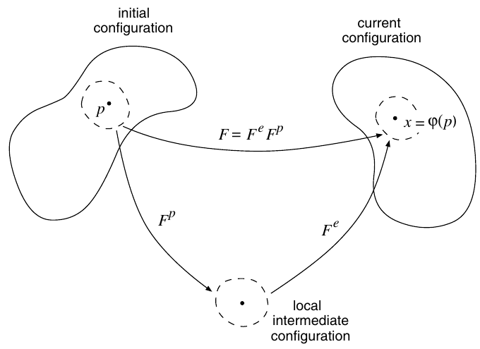
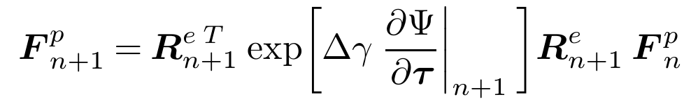
The crucial difference between the discretisation of the large strain problem and the infinitesimal one lies in the numerical approximation of the plastic flow equation. The structure of the plastic flow equation makes algorithms based on exponential map integrators.
How to use it?
This Constitutive law has some checks in order to verify that all the parameters are provided but, very briefly, we are going to describe those parameters in order to perform a calculation. The generic StructuralMaterials.json has the following structure:
{
        "model_part_name" : "Parts_Shell",
        "properties_id"   : 1,
        "Material"        : {
            "constitutive_law" : {
                "name" : "SmallStrainIsotropicPlasticityFactory3D",
                "yield_surface" :  "VonMises",
                "plastic_potential" : "VonMises"
            },
            "Variables"        : {
                "DENSITY"       : 7850.0,
                "YOUNG_MODULUS" : 206900000000.0,
                "POISSON_RATIO" : 0.29,
                "YIELD_STRESS_TENSION" : 275.0e6,
                "YIELD_STRESS_COMPRESSION" : 275.0e6,
                "FRACTURE_ENERGY" : 1.0e5,
                "HARDENING_CURVE" : 1,
                "MAXIMUM_STRESS" : 300.0e6,
                "MAXIMUM_STRESS_POSITION" : 0.3
            },
            "Tables"           : {}
        }
    }
The parameters needed for the plasticity (neglecting the young modulus and poisson ratio) are (use International System):
- yield_surface : Defines the yield surface to use
- plastic_potential : Defines the plastic potential to use
FRACTURE_ENERGY: Defines the maximum energy that the system can dissipate at each integration pointYIELD_STRESS_COMPRESSION: Maximum yield strength in compressionYIELD_STRESS_TENSION: Maximum yield strength in tensionHARDENING_CURVE: Defines the flow rule to use (LinearSoft=0, ExpSoft=1, Hardening=2, PerfPlast=3)MAXIMUM_STRESS_POSITION: ONLY FOR CURVE 2, Defines the position of the peak strength (value ranging 0-1)MAXIMUM_STRESS: ONLY FOR CURVE 2, Defines the peak strength valueFRICTION_ANGLE: Defines the friction angle value in degreesDILATANCY_ANGLE: Defines the dilatancy angle value in degrees (usually 0.5*friction_angle)
Small Strain Isotropic Damage
General Description
Continuum damage mechanics is a branch of continuum mechanics that describes the progressive loss of material integrity due to the propagation and coalescence of micro-cracks, micro-voids, and similar defects. These changes in the microstructure lead to an irreversible material degradation, characterized by a loss of stiffness that can be observed on the macro-scale.
The structure of the damage constitutive law is analogous to the plasticity case. Indeed, the damage constitutive law (generic_small_strain_isotropic_plasticity.cpp) has a template of an integrator that calculates the damage internal variable and computes the integrated or real stress according to the degradation of the material. This damage CL uses the Yield Surfaces previously described in an identical way as the plasticity. If you want more information about the template structure I recommend you to see the plasticity chapter where it is detailed.
How to use it?
The general StructuralMaterials.json have the following structure:
{
        "model_part_name" : "Parts_Shell",
        "properties_id"   : 1,
        "Material"        : {
            "constitutive_law" : {
                "name" : "SmallStrainIsotropicDamageFactory3D",
                "yield_surface" :  "VonMises"
                "plastic_potential" : "VonMises"
            },
            "Variables"        : {
                "DENSITY"       : 7850.0,
                "YOUNG_MODULUS" : 206900000000.0,
                "POISSON_RATIO" : 0.29,
                "YIELD_STRESS_TENSION" : 275.0e6,
                "YIELD_STRESS_COMPRESSION" : 275.0e6,
                "FRICTION_ANGLE" : 32.0,
                "SOFTENING_TYPE" : 1
            },
            "Tables"           : {}
        }
}
The parameters are the following (use International System):
- yield_surface : Defines the yield surface to use
- plastic_potential : Defines the plastic potential to use (not used in damage)
FRACTURE_ENERGY: Defines the maximum energy that the system can dissipate at each integration pointYIELD_STRESS_COMPRESSION: Maximum yield strength in compressionYIELD_STRESS_TENSION: Maximum yield strength in tensionFRICTION_ANGLE: Defines the friction angle value in degreesSOFTENING_TYPE: Defines the softening type (linear softening=0, exponential softening=1)
Small Strain d+d- Damage
General Description
In this case, we have implemented a more sophisticated damage model that differentiates the behaviour of the material depending on the sign of the stresses. In other words, the damage behaviour is different in compression and tension. This is done by performing an Spectral Decomposition of the Stress Tensor (see constitutive_law_utilities.cpp) in which we separate the tension/compression states [2,3].
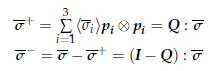
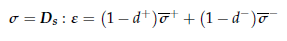
Once we have Decomposed the stress tensor we proceed to the calculation of the damage variables (now d+ and d- corresponding to the tension/compression damage) and compute the integrated stress tensor as:
In order to guarantee flexibility, we have designed an structure capable of combining different yield surfaces in tension and in compression. This has been achieved by templating two integrators named TConstLawIntegratorTensionType and TConstLawIntegratorCompressionType which define the tension/compression yield surfaces and flow rules.
The implementation is described below (generic_small_strain_d_plus_d_minus_damage.cpp):
template <class TConstLawIntegratorTensionType, class TConstLawIntegratorCompressionType>
class KRATOS_API(STRUCTURAL_MECHANICS_APPLICATION) GenericSmallStrainDplusDminusDamage
How to use it?
The general StructuralMaterials.json has the following form:
{
        "model_part_name" : "Parts_Shell",
        "properties_id"   : 1,
        "Material"        : {
            "constitutive_law" : {
                "name" : "SmallStrainDplusDminusDamageModifiedMohrCoulombVonMises3D"
            },
            "Variables"        : {
                "DENSITY" : 7850.0,
                "YOUNG_MODULUS" : 206900000000.0,
                "POISSON_RATIO" : 0.29,
                "FRACTURE_ENERGY" : 1.5e2,
                "FRACTURE_ENERGY_COMPRESSION" : 1.0e2,
                "YIELD_STRESS_TENSION" : 3.0e6,
                "YIELD_STRESS_COMPRESSION" : 1.0e6,
                "FRICTION_ANGLE" : 32.0,
                "DILATANCY_ANGLE" : 16.0,
                "SOFTENING_TYPE" : 1
            },
            "Tables"           : {}
        }
}
The parameters required for this model have been explained previously and the way of combining yield surfaces is by calling the already registered combinations of them. For instance, in this example the name of the law is SmallStrainDplusDminusDamageModifiedMohrCoulombVonMises3D so it means that we are using a d+d- damage model using a Modified Mohr Coulomb yield surface for tension and Von Mises for compression. In this way we define the combinations by typing as “name”:
SmallStrainDplusDminusDamage<TensionYieldSurface,CompressionYieldSurface>3D and the yield surfaces (keywords) available are, as explained before:
- Rankine
- Tresca
- VonMises
- ModifiedMohrCoulomb
- DruckerPrager
- SimoJu
- Classical Mohr-Coulomb
ViscoElasticity
General Description
One of the behaviors responsible for the nonlinearity in the materials’ response over the time field is due to viscoelasticity. Viscoelasticity studies the rheological behavior of materials, in other words, behaviors affected by the course of time.
Up to now, we have developed two viscous models: the Generalized Maxwell model (used to simulate the stress relaxation of materials) and the Generalized Kelvin model (used to simulate creep and delayed strains).
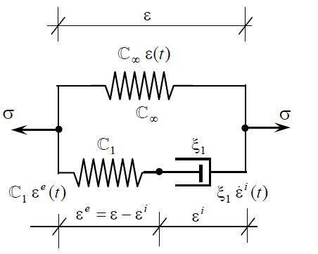
Generalized Maxwell model
This viscoelastic model has been widely used when simulating the stress relaxation of materials subjected to a constant strain rate (like in pre-stressing tendons used in civil engineering). The spring-damper diagram is (see [1] for more information) as follows:
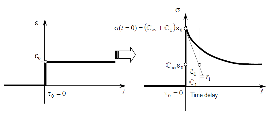
And the general behaviour of the model can be seen in the picture below [1]:
How to use it?
The general StructuralMaterials.json have the following structure:
{
        "model_part_name" : "Parts_Shell",
        "properties_id"   : 1,
        "Material"        : {
            "constitutive_law" : {
                "name" : "ViscousGeneralizedMaxwell3D"
            },
            "Variables"        : {
                "DENSITY"       : 7850.0,
                "YOUNG_MODULUS" : 206900000000.0,
                "POISSON_RATIO" : 0.29,
                "VISCOUS_PARAMETER" : 0.15,
                "DELAY_TIME" : 1.0
            },
            "Tables"           : {}
        }
}
The parameters are the following:
DELAY_TIME: Defines the initial slope of the curve (see previous figure)VISCOUS_PARAMETER: Is the ratio between the stiffnesses C1/Cinf
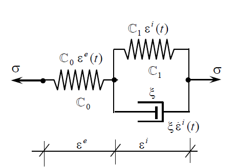
Generalized Kelvin model
This viscous model has been used in general to simulate delayed strains in materials such as the creep in concrete and soils. The spring-damper diagram is (see [1] for more information) as follows:
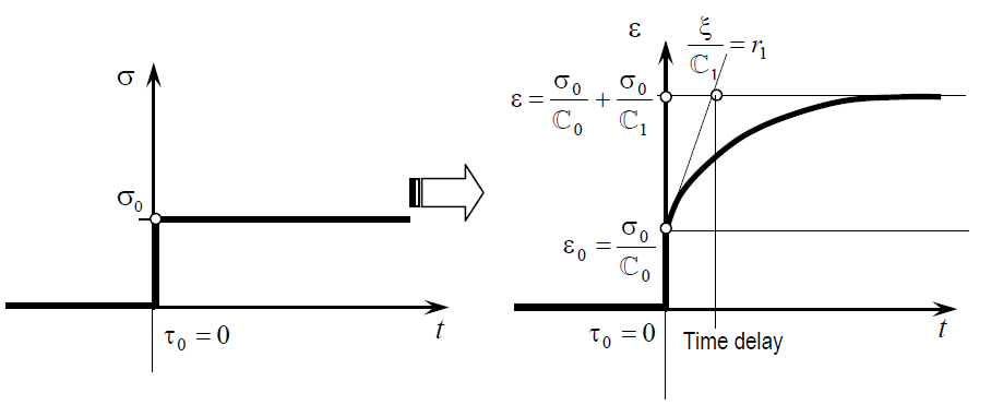
And the general behaviour of the model can be seen in the picture below [1]:
How to use it?
The general StructuralMaterials.json have the following structure:
{
        "model_part_name" : "Parts_Shell",
        "properties_id"   : 1,
        "Material"        : {
            "constitutive_law" : {
                "name" : "ViscousGeneralizedKelvin3D"
            },
            "Variables"        : {
                "DENSITY"       : 7850.0,
                "YOUNG_MODULUS" : 206900000000.0,
                "POISSON_RATIO" : 0.29,
                "DELAY_TIME" : 150.0
            },
            "Tables"           : {}
        }
}
The parameters are the following:
DELAY_TIME: Defines the initial slope of the curve (see previous figure)
ViscoPlasticity
In this case we were seeking a constitutive law that allows the material to develop plastic strains as well as a certain stress relaxation along time. This can be achieved with the formulation proposed but some other procedures will be implemented to increase the variety and polivalence of the Structural Mechanics Application.
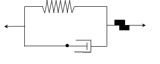
The spring damper scheme for this methodology is shown below and allows the material to plastify and, in a viscous way, relax the stress along time.
Appendix
The Mohr-Coulomb modified yield surface
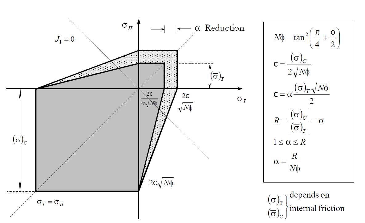
The Mohr-Coulomb function cannot be used directly in frictional cohesive materials such as concrete, which has an internal friction angle of φ≅32 According to the Mohr- Coulomb classic formulation, a limit strength relation is obtained for this angle between a traction behavior and a uniaxial compression behavior of tan[(π / 4) + (φ / 2)]= 3,25. This magnitude is very different from the concrete magnitude, which should be around 10. To solve this problem, either the friction angle can be increased causing a dilatancy excess or the original criterion can be modified. By this last option, the following expression is obtained,
F(σ) = f(σ) - c
where the stress function “f” is expressed as[1] (being θ the Lode’s angle, I1, J2 the classical stress invariants and φ the friction angle):
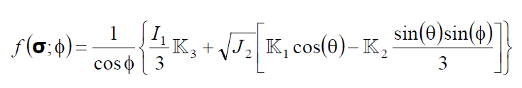
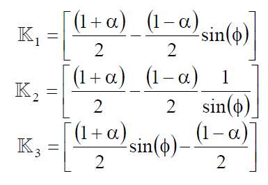
Through this new Mohr-Coulomb modified function any strength relation required by the different materials can be established by only modifying Ki , without increasing dilatancy.
The values of the Ki and the parameters required can be seen in the figures below[1].
References
[1] “Dinámica no lineal” by S. Oller.
[2] “An Energy-Equivalent d+/d- Damage Model with Enhanced Microcrack Closure-Reopening Capabilities for Cohesive-Frictional Materials” by M. Cervera and C.Tesei.
[3] “A Strain-Based Plastic Viscous-Damage Model for Massive Concrete Structures” by R. Faria, J. Oliver and M. Cervera.
[4] “Computational methods for plasticity. Theory and applications” by EA de Souza Neto, D Perić and DRJ Owen
[5] “Non-linear Finite Elements for continua and structures” by Ted Belytschko, Wing Kam Liu, Brian Moran and Khalil I. Elkhodary
Contact us!
If you have any doubts about the Constitutive Laws in the Structural Mechanics Application do not hesitate to contact us at acornejo@cimne.upc.edu and vmataix@cimne.upc.edu.