Manipulating solution values
Objective
To apply a parabolic (space dependent) inlet (pointing in positive X direction) on the CFD domain by accessing and setting the VELOCTIY variable. The magnitude of the velocity inlet varies with time with the following relation
VELOCITY_X = (25.0*TIME)/(10.0)
The equation for the parabolic inlet profile is
VELOCITY_X = VELOCITY_X * ( (y * y)/(600 * 600) )
1. Introduction
This tutorial session is intended to illustrate how the Kratos’ data structure, when accessed form Python, can be used to manipulate and set custom boundary conditions, solutions over the computational domain in a given problem. The following explanation builds upon the previous sessions of Data management and Solving strategies.
Here the CFD problem described in the first tutorial of Running an example from GiD is used as the working example. The setup files (mdpa, MainKratos.py and the JSON) of this problem can be downloaded from here. Please extract the zip file and make it ready for the next task.
2. The CFD example
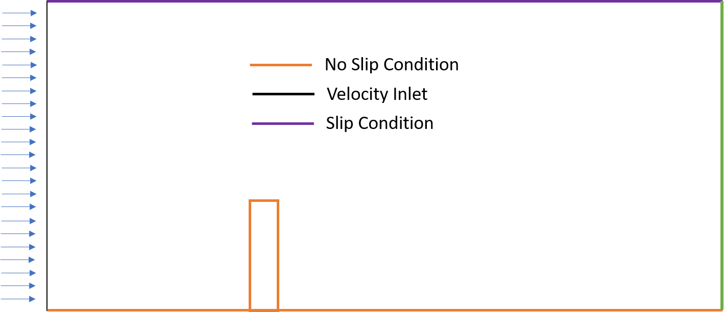
As the first step of this tutorial, we understand the CFD example problem setup and run the simulation to observe the initial result. The CFD problem setup is illustrated below

As illustrated, a no slip condition is applied on the top and bottom walls of the 2D fluid domain. A uniform and constant velocity inlet is applied on the left hand side and a pressure outlet (0 pressure) is applied on the right hand side of the domain. These boundary condition are defined in the ProjectParameters.json. The following lines from the ProjectPrameters.json reflect the same
       "boundary_conditions_process_list" : [{
            "python_module" : "apply_inlet_process",
            "kratos_module" : "KratosMultiphysics.FluidDynamicsApplication",
            "Parameters"    : {
                "model_part_name" : "FluidModelPart.AutomaticInlet2D_Inlet",
                "variable_name"   : "VELOCITY",
                "modulus"         : "25.0*t/10.0",
                "direction"       : "automatic_inwards_normal",
                "interval"        : [0,10.0]
            }
        },{
            "python_module" : "apply_inlet_process",
            "kratos_module" : "KratosMultiphysics.FluidDynamicsApplication",
            "Parameters"    : {
                "model_part_name" : "FluidModelPart.AutomaticInlet2D_Inlet",
                "variable_name"   : "VELOCITY",
                "modulus"         : 25.0,
                "direction"       : "automatic_inwards_normal",
                "interval"        : [10.0,"End"]
            }
        },{
            "python_module" : "apply_outlet_process",
            "kratos_module" : "KratosMultiphysics.FluidDynamicsApplication",
            "Parameters"    : {
                "model_part_name"    : "FluidModelPart.Outlet2D_Outlet",
                "variable_name"      : "PRESSURE",
                "constrained"        : true,
                "value"              : 0.0,
                "hydrostatic_outlet" : false,
                "h_top"              : 0.0
            }
        },{
            "python_module" : "apply_noslip_process",
            "kratos_module" : "KratosMultiphysics.FluidDynamicsApplication",
            "Parameters"    : {
                "model_part_name" : "FluidModelPart.NoSlip2D_InterfaceFluid"
            }
        },{
            "python_module" : "apply_slip_process",
            "kratos_module" : "KratosMultiphysics.FluidDynamicsApplication",
            "process_name"  : "ApplySlipProcess",
            "Parameters"    : {
                "model_part_name" : "FluidModelPart.Slip2D"
            }
        }]
More information on which processes exists for boundary conditions and how to use them is described in this wiki page.
Please run the example by using the method described in the previous tutorials. That is by using the python executable. Once the simulation is finished we load the result (.bin) file into GiD to view the following result

3. The MainKratos.py Script
This is the script that instantiates the fluid dynamics analysis and calls the Run function of the solver class to solve the CFD problem with applied boundary conditions.
import KratosMultiphysics
from KratosMultiphysics.FluidDynamicsApplication.fluid_dynamics_analysis import FluidDynamicsAnalysis

import sys
import time

class FluidDynamicsAnalysisWithFlush(FluidDynamicsAnalysis):

    def __init__(self,model,project_parameters,flush_frequency=10.0):
        super(FluidDynamicsAnalysisWithFlush,self).__init__(model,project_parameters)
        self.flush_frequency = flush_frequency
        self.last_flush = time.time()

    def FinalizeSolutionStep(self):
        super(FluidDynamicsAnalysisWithFlush,self).FinalizeSolutionStep()

        if self.parallel_type == "OpenMP":
            now = time.time()
            if now - self.last_flush > self.flush_frequency:
                sys.stdout.flush()
                self.last_flush = now

if __name__ == "__main__":

    with open("ProjectParameters.json",'r') as parameter_file:
        parameters = KratosMultiphysics.Parameters(parameter_file.read())

    model = KratosMultiphysics.Model()
    simulation = FluidDynamicsAnalysisWithFlush(model,parameters)
    simulation.Run()
As we see here, a custom fluid dynamics analysis is derived from the actual FluidDynamicsAnalysis to make a FluidDynamicsAnalysisWithFlush class and uses it for the simulation.
This FluidDynamicsAnalysisWithFlush can be used to modify the properties of the simulation, even those specified in the JSON file.
4. Accessing the sub-modelpart of the inlet boundary
The sub-modelparts can be accessed from the model, which is stored in the base fluid dynamics analysis. The following lines of python code
self.inlet_sub_modelpart = self.model['FluidModelPart.AutomaticInlet2D_Inlet']
will fetch the sub-modelpart and gives access to the entities (nodes, conditions) on the inlet. In this problem, since the inlet is a line, we will have nodes and line conditions. Knowing this, now the question is where do we access and set the parabolic inlet boundary condition. For this we first save the inlet_sub_modelpart in the FluidDynamicsAnalysisWithFlush this is done by overriding the Initialize function of the base fluid dynamics analysis as follows
def Initialize(self):
    super(CustomFluidDynamicsAnalysis, self).Initialize()
    self.inlet_sub_modelpart = self.model['FluidModelPart.AutomaticInlet2D_Inlet']
5. Computing and setting the inlet boundary condition
Since the inlet boundary condition is changing every time step, the magnitude is to be reset at the beginning of every time step. This requires the InitializeSolutionStep function of the fluid dynamics analysis is to be overridden and we set the inlet velocity in this function.
    def InitializeSolutionStep(self):
        super(CustomFluidDynamicsAnalysis, self).InitializeSolutionStep()
        for node in self.inlet_sub_modelpart.Nodes:
            #x = node.X
            y = node.Y
            #z = node.Z
            # Obtaining the current velocity magnitude (since here only VELOCTY is [1,0,0])
            current_x_vel = node.GetSolutionStepValue(KratosMultiphysics.VELOCITY_X)
            # Calculate the new velocity magnitude
            modified_x_vel = current_x_vel * ((y*y) / (600*600))
            #modified_x_vel = current_x_vel
            # Setting new solution on the node
            node.SetSolutionStepValue(KratosMultiphysics.VELOCITY_X,0,modified_x_vel)
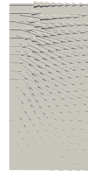
Once the simulation is done with this modification, we see the following profile on the inlet of the domain
