Edit me

Multiphysics example

Objective

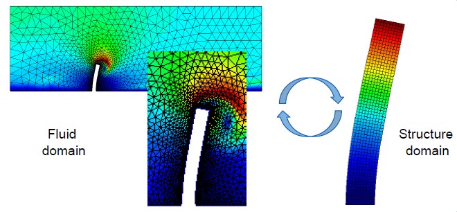
The main goal is to become familiar with key aspects of multiphysics simulations using a prototypical example. The chosen problem is a case of fluid-structure interaction. One should become familiar with the various components involved in setting up and running such simulations, as well as the necessary steps to ensure the quality and physical relevance of results.

The first example will be used in a black-box manner to discuss the most important details related to setting up such cases and the corresponding parameters. The second example depicts how one could create own - so customized - mapping and solvers to further enhance existing capabilities.

Suggestion: as soon as you are here, you should download the source files and start running the respective simulations from the command line as explained in Kratos input files and IO (section 2.2: Run Kratos from the command line) . As there are 2 examples intended to be shown, it would be sufficient if every other person would run one and the remaining participants the other, preferably in groups of two.

Simulation 1: in 6_multiphysics\FSIBlackboxGeneric\MainKratos.py
Simulation 2: in 6_multiphysics\FSICustomizedSDoFVortexShedding\MainKratosFSI.py

1. FSI Black-box generic

The discussion relies on the examples discussed in Running an example from GiD. Here it was shown how a CFD (section 3) and a CSM (section 4) can be set up and run. Additionally, in section 5 an FSI example was provided which builds upon the CFD and CSM setups.

For this you should download and refer to the input files for the respective case.

The main components of this certain multiphysics case - an FSI simulation - are:

the CFD “simulation”: model part KratosWorkshop2019_high_rise_building_FSI_Fluid.mdpa and respective settings "structure_solver_settings"
the CSM “simulation” : model part KratosWorkshop2019_high_rise_building_FSI_Structural.mdpa and respective settings "fluid_solver_settings"

The settings are now all contained in one file, the ProjectParameters.json:

    "solver_settings"  : {
        "solver_type"               : "Partitioned",
        "coupling_scheme"           : "DirichletNeumann",
        "echo_level"                : 1,
        "structure_solver_settings" : {...},
        "fluid_solver_settings"     : {...},
        "mesh_solver_settings"      : {...},
        "coupling_settings"         : {...}

As it can be observed that there are more settings blocks, as additional components are needed to enable the proper functioning.

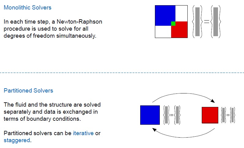
the solver type: when referring to multiphysics simulations, one generally tries to deal with a complex problem, which can be solved in various manners: either monolithic (which leads to one large system to be solved) or partitioned (which implies splitting up the problem into dedicated fields, dealing with these separately and ensuring proper data transfer and convergence

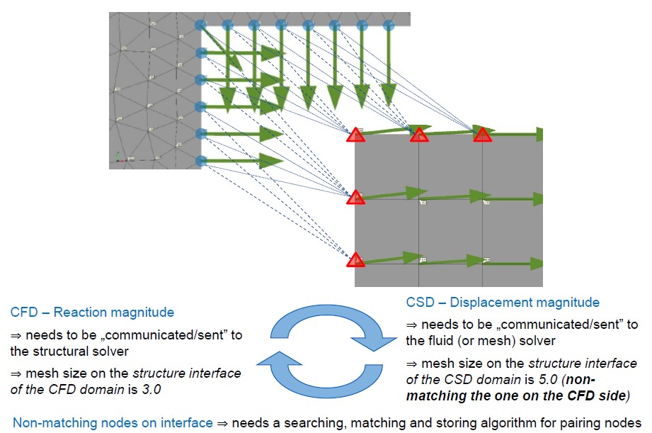
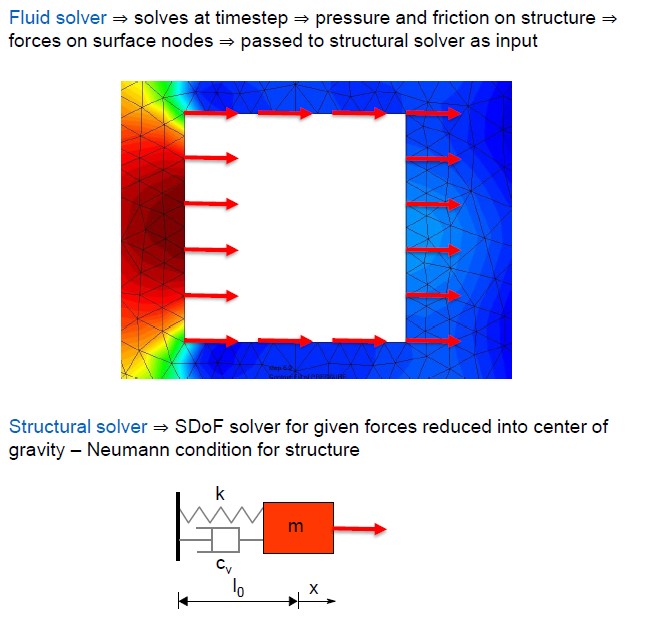
the coupling scheme: here a Dirichlet-Neumann-type coupling is used, which specifies which values are affected by the mapping, more precisely for this case: the CFD simulation results in fluid forces on the respective structure interface, these forces being transferred (mapped) onto the structure and serving as the right hand side (RHS - or force vector), so as a Neumann boundary condition for the CSM; the CSM solve results in the deformation of the structural model, the deformations from the boundary to the fluid are transferred (mapped) onto the CFD domain, these deformations serving affecting the left hand side (LHS - or the vector of primary variables) for the pseudo-structural problem (refer to the next point of the mesh solver), constituting a Dirichlet boundary condition

the mesh solver and its settings: this builds upon the existing parts of the CFD (see the provided "model_part_name") and is responsible for deforming the CFD mesh in order to consistently match the deformations on the interface of the fluid to the structure, which is done using a pseudo-structural formulation (hinted by the naming of the "solver_type"), as the mesh deformations are solved as if this was a structural mechanics problem with prescribed deformations on the respective boundary

"mesh_solver_settings"      : {
          "echo_level"      : 0,
          "domain_size"     : 2,
          "model_part_name" : "FluidModelPart",
          "solver_type"     : "structural_similarity"
      },

Note: the mesh solver will require additional boundary conditions. For this particular case, the nodes on the inlet, top, bottom and outlet will need to have a prescribed value for (mesh) displacement of zero. These can be seen in the respective blocks of the project parameters (in the "fluid_boundary_conditions_process_list"), such as:

{
          "python_module" : "assign_vector_variable_process",
          "kratos_module" : "KratosMultiphysics",
          "Parameters"    : {
              "model_part_name" : "FluidModelPart.ALEMeshDisplacementBC2D_FluidALEMeshBC",
              "variable_name"   : "MESH_DISPLACEMENT",
              "constrained"     : [true,true,true],
              "value"           : [0.0,0.0,0.0],
              "interval"        : [0.0,"End"]
          }
      }

where ALE stands for the Arbitrary-Lagrangian-Eulerian formulation.

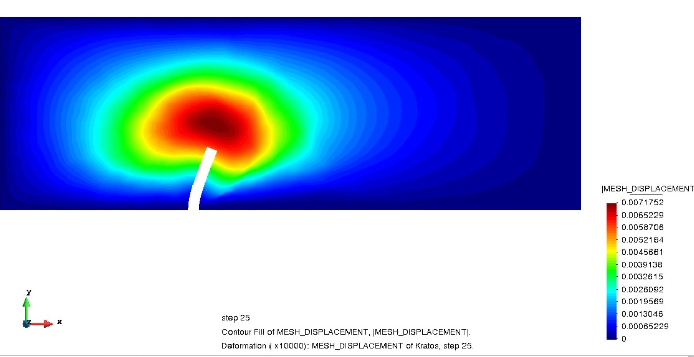
the coupling and its settings: coupling the above solver is done in an partitioned manner using iterations to lead to convergence; it is important to note the "mapper_settings", which is responsible for providing the necessary information to setup and carry out the mapping (transfer) of necessary data fields; "coupling_strategy_settings" defines the way the inner iterations are done to achieve convergence at the interface; additionally the correct sub model parts need to provided - "structure_interfaces_list" and "fluid_interfaces_list"

    "coupling_settings"         : {
          "nl_tol"                       : 1e-6,
          "nl_max_it"                    : 15,
          "solve_mesh_at_each_iteration" : true,
          "mapper_settings"              : [{
              "mapper_face"                           : "unique",
              "fluid_interface_submodelpart_name"     : "FluidNoSlipInterface2D_InterfaceFluid",
              "structure_interface_submodelpart_name" : "StructureInterface2D_InterfaceStructure"
          }],
          "coupling_strategy_settings"   : {
              "solver_type"       : "Relaxation",
              "acceleration_type" : "Aitken",
              "w_0"               : 0.825
          },
          "structure_interfaces_list"    : ["StructureInterface2D_InterfaceStructure"],
          "fluid_interfaces_list"        : ["FluidNoSlipInterface2D_InterfaceFluid"]
      }

Once the simulation is done, the (mesh) displacement results should be viewed.

For the CFD partition it looks like this:

For the CSM partition:

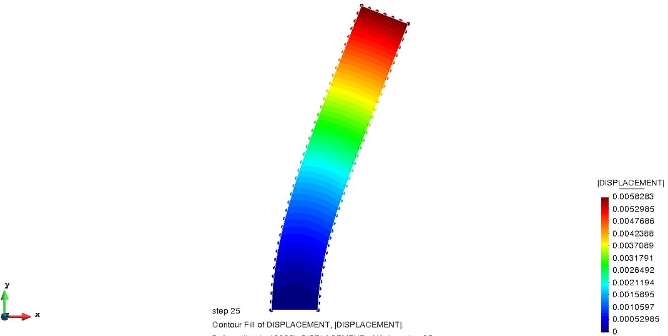
One can observe that the deformation of the two domains is consistent. This suggests the proper choice of settings for convergence. This example uses the capabilities of KratosMultiphysics as a black-box. The problem definition setup can be done, for e.g. in GiD. After the creation of the model parts and the initial settings, the user might want or need to change settings in the parameters file to re-run.

2. FSI Customized SDoF vortex shedding

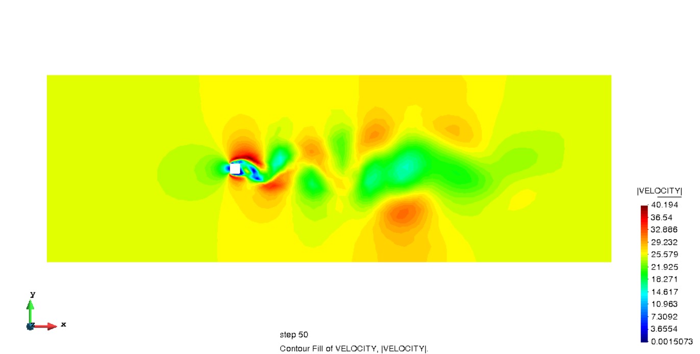
This example is chosen to show how one could additionally use own - custom python scripts to achieve coupling. The underlying CFD case is that of a rectangular cylinder in constant flow. Harmonic forces arise perpendicular to the flow due to vortex shedding. A single-degree-of-freedom (SDoF) structural model is chosen as the custom CSM solver.

The CFD case results - vortex shedding results can be seen:

For this problem, the SDoF solver is chosen to model the rigid body displacement of the square perpendicular to the flow direction, which leads to the following setup for the FSI:

The necessary parameters files are:

ProjectParametersCFD.json : contains all necessary information to setup and run the CFD simulation, as well as the additional mesh moving prerequisites

ProjectParametersCSM.json : contains all necessary information to setup and run the CSM simulation (here an SDoF oscillator)

{
  "problem_data": {
      "problem_name": "CSM",
      "time_step": 0.05,
      "start_time": 0.0,
      "end_time": 50
  },
  "model_data": {
      "absolute_position": 0.0,
      "mass": 1e7,
      "eigen_freq": 0.1,
      "zeta": 0.05,
      "rho_inf": 0.16,
      "initial": {
          "displacement": 0.0,
          "velocity": 0.0,
          "acceleration": 0.0
      },
      "dof_type": "DISPLACEMENT_Y"
  }
}

ProjectParametersFSI.json : contains all necessary information to setup the mapping and coupling

{
  "problem_data"             : {
      "problem_name"    : "FSI",
      "time_step"       : 0.05,
      "start_time"      : 0.0,
      "end_time"        : 50,
      "echo_level"      : 1
},
  "coupling_settings":{
          "mapper_settings":{
          "mapper_type": "sdof",
          "interface_submodel_part_destination": "NoSlip2D_structure",
          "interface_submodel_part_origin": "SDoF_origin"
       },
       "convergence_accelerator_settings": {
          "type": "aitken",
          "max_iterations": 5,
          "residual_relative_tolerance": 1e-5,
          "residual_absolute_tolerance": 1e-9,
          "relaxation_coefficient_initial_value": 0.25
      }
  }
}

The necessary customized python implementation are:

the CSM solver: python code in structure_sdof_solver.py; this has a similar code structure as the application in KratosMultiphysics;

class StructureSDoF(object):
    # Direct time integration of linear SDOF (Generalized-alpha method).
    # This class takes the undamped eigenfrequency (f, [Hz]) as input
    def GetDisplacement(self):
    def SetDisplacement(self, displacement):
    def Predict(self):
    def PrintSupportOutput(self):
    def SetExternalForce(self, ext_force):
    def _AssembleLHS(self):
    def _AssembleRHS(self):
    def FinalizeSolutionStep(self):
    def SolveSolutionStep(self):
    def _IncrementTimeStep(self):
    def Initialize(self):
    def Finalize(self):
    def InitializeSolutionStep(self):
    def AdvanceInTime(self, time):
    def OutputSolutionStep(self):
    def GetPosition(self):

the FSI utilities (like mapper and convergence accelerator): python code in fsi_utilities.py ```python
functionalities related to mapping

def GetDisplacements(structure_solver): def SetDisplacements(displacements, structure_solver): def NeumannToStructure(mapper, structure_solver, flag): def DisplacementToMesh(mapper, displacement, structure_solver):

def CreateMapper(destination_model_part, mapper_settings):

class CustomMapper(object):

def CreateConvergenceAccelerator(convergence_accelerator_settings):

class ConvergenceAcceleratorBase(object): def CalculateResidual(self, solution, old_solution): def CalculateRelaxedSolution(self, relaxation_coefficient, old_solution, residual): def ComputeRelaxationCoefficient(self):

class AitkenConvergenceAccelerator(ConvergenceAcceleratorBase): def ComputeRelaxationCoefficient(self, old_coefficient, residual, old_residual, iteration,

* the **main script**: python code in `MainKratosFSI.py`; it is written in a way that it follows the KratosMultiphysics code structure and accommodates the custom python scripts
```python
'''
The initial part takes care of reading in the project parameters and initializing the models
Here we only present the main structure of the computation loop
'''

while(time <= end_time):
    new_time_fluid = fluid_solver._GetSolver().AdvanceInTime(time)
    new_time_structure = structural_solver.AdvanceInTime(time)

    fluid_solver._GetSolver().Predict()
    structural_solver.Predict()

    fluid_solver.InitializeSolutionStep()
    structural_solver.InitializeSolutionStep()

    time = time + delta_time

    residual = 1
    # from the nodes in the structure (origin) on the interface
    old_displacements = fsi_utilities.GetDisplacements(structural_solver)

    num_inner_iter = 1
    ### Inner FSI Loop (executed once in case of explicit coupling)
    for k in range(convergence_accelerator.max_iter):

        fsi_utilities.DisplacementToMesh(mapper, old_displacements, structural_solver)

        # Mesh and Fluid are currently solved independently, since the ALE solver does not copy the mesh velocity
        # Solve Mesh
        fluid_solver._GetSolver().SolveSolutionStep()

        fsi_utilities.NeumannToStructure(mapper, structural_solver, True)

        # Solver Structure
        structural_solver.SolveSolutionStep()

        # Convergence Checking (only for implicit coupling)
        if convergence_accelerator.max_iter > 1:
            displacements = fsi_utilities.GetDisplacements(structural_solver)

            # Compute Residual
            old_residual = residual
            residual = convergence_accelerator.CalculateResidual([displacements], [old_displacements])

            if (fsi_utilities.Norm(residual) <= convergence_accelerator.res_rel_tol):
                fsi_utilities.SetDisplacements(displacements, structural_solver)

                print("******************************************************")
                print("************ CONVERGENCE AT INTERFACE ACHIEVED *******")
                print("******************************************************")
                break
            else:
                relaxation_coefficient = convergence_accelerator.ComputeRelaxationCoefficient(relaxation_coefficient, residual, old_residual, k)
                relaxed_displacements = convergence_accelerator.CalculateRelaxedSolution(relaxation_coefficient, [old_displacements], residual)[0]
                old_displacements = relaxed_displacements
                fsi_utilities.SetDisplacements(relaxed_displacements, structural_solver)

                num_inner_iter += 1

            if (k+1 >= convergence_accelerator.max_iter):
                print("######################################################")
                print("##### CONVERGENCE AT INTERFACE WAS NOT ACHIEVED ######")
                print("######################################################")

            print("==========================================================")
            print("COUPLING RESIDUAL = ", fsi_utilities.Norm(residual))
            print("COUPLING ITERATION = ", k+1, "/", convergence_accelerator.max_iter)
            print("RELAXATION COEFFICIENT = ", relaxation_coefficient)
            print("==========================================================")


    fluid_solver.FinalizeSolutionStep()
    structural_solver.FinalizeSolutionStep()

    fluid_solver.OutputSolutionStep()
    structural_solver.OutputSolutionStep()

    disp = structural_solver.GetDisplacement()
    file_writer.WriteToFile([time, disp, num_inner_iter])

fluid_solver.Finalize()
structural_solver.Finalize()

file_writer.CloseFile()

The results for the CFD domain with mesh moving - (mesh) displacement y of the upper left corner of the square (opening MainModelPart.post.bin in GiD):

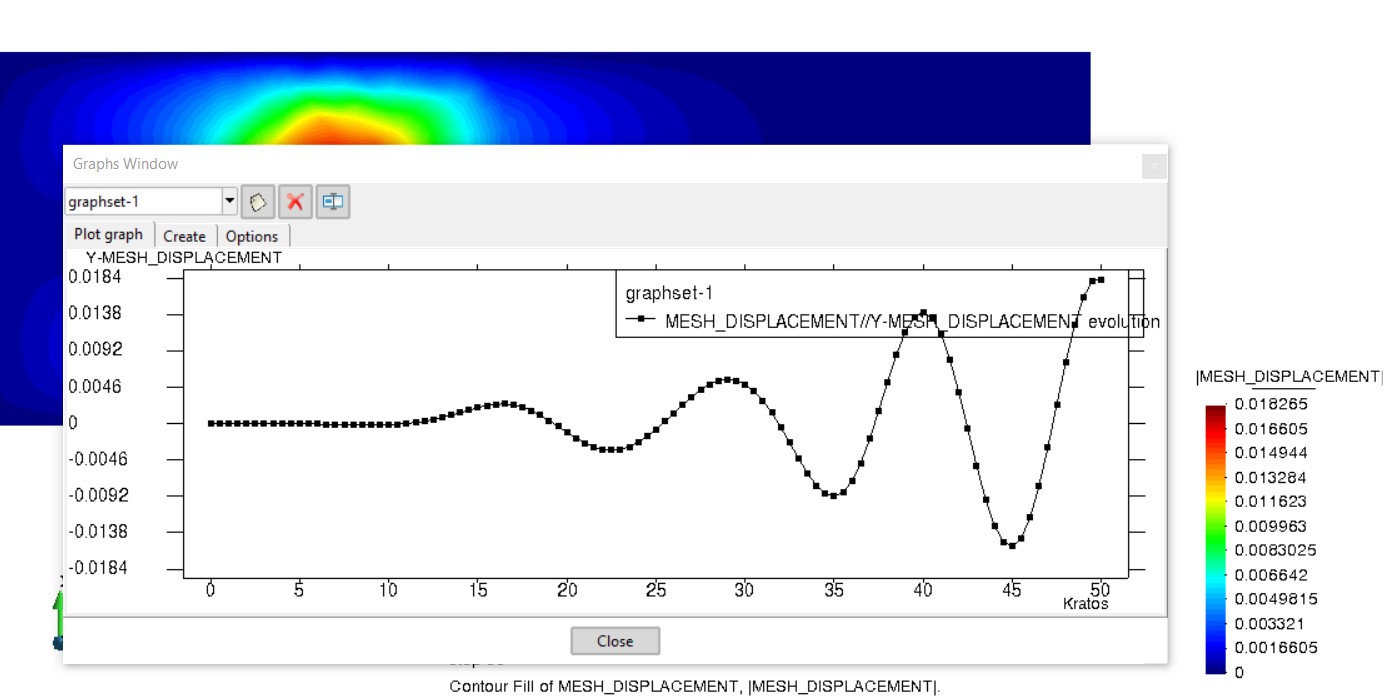
The results for the CSM solver plotted with python (using the provided plot_displacement_results.py) from the resulting ascii file sdof_csm_displacement_y.dat:

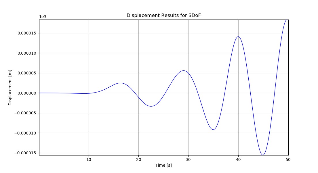
The goal of the second example is to show you how you could take one or more existing applications from KratosMultiphysics and coupling these in a customized manner, also including own solver, both carried out in the python layer.

Sources: The image related to monolithic-partitioned manner is adapted from: W.G. Dettmer: On Partitioned Solution Strategies for Computational Fluid-Structure Interaction. Other images and material is taken from and based upon the lecture content of Structural Wind Engineering WS18-19, Chair of Structural Analysis @ TUM - R. Wüchner, M. Péntek.

Multiphysics Example

Multiphysics example

Objective

1. FSI Black-box generic

2. FSI Customized SDoF vortex shedding

functionalities related to mapping

functionalities related to the convergence accelerator