Introduction
Explicit Vertex morphing (here onwards called as vertex morphing) is a discrete filtering method to regularize optimization problem. Non-smooth discrete gradient field is a common challenge in optimization problems which makes design updates noisy and non-applicable for numerical model, for instance, bad elements which eventually result in failure in primal and adjoint solution computation. Therefore it is crucial to apply a filtering technique to obtain a smooth design updates. An example of a noisy field is shown in figure 1.
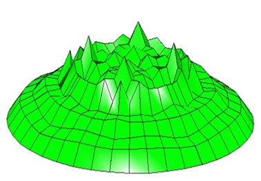
Figure 1: Noisy design field
Definition
Figure 2 illustrates the filtering methodology applied in vertex morphing. Control field (i.e. sensitivity field) is demonstrated by \(S\left(\xi\right)\). Filtering domain is identified by the used \(r\) filter radii for each mesh coordinate. Then a filtering function of \(A\left(\xi-\xi_0\right)\) is applied on the filtering domain to obtain smoothened and filtered design control field of \(z\left(\xi_o\right)\) as illustrated in the figure.
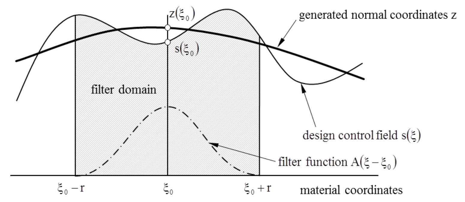
Figure 2: Vertex morphing filtering
Following equation is used to obtain the final filtered design control field.
$$ z\left(x_0\right) = \int_{x_0-r}^{x_0+r} A\left(x, x_0, r\right)s\left(x\right) d\Gamma $$
Figure 2 illustrates obtained filtered and smoothened design field of the noist design field illustrated in figure 1.

Figure 2: Filtered design field
It is important to note that the variability of the resulting shape is characterized by the density of the design grid used to discretize the physical field \(s\). The filter helps to control the continuity properties of the resulting shape. The filter does not affect the global and local solutions and leaves them unchanged. Typically, of course, in the case of non-convex problems different local solutions are found for different filters as they modify the descent directions. The physical space and its variety of alternative local optima are easily explored with repeated optimization and varied filters.
Effect of filter radii
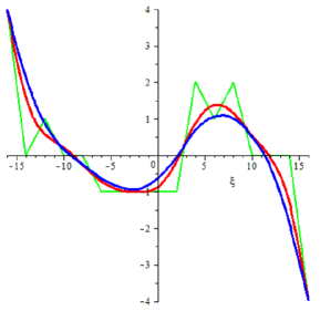
Higher filter radii (i.e. \(r\)) results in smoothened design field over a circular area in 2D and a spherical area in 3D with radius \(r\). It may loose the local effect which are significant in obtaining design field which is capable of optimizing the given objective(s). This is illustrated in figure 3. In there, green plot illustrates the noisy design field in physical space, blue plot illustrates filtered design field in control space with \(r=4\) and red plots illustrate filtered design fields with \(r=6\) (left) and \(r=16\) (right).
![]()
Figure 3: Filter radii effect on smoothened design field
Filter functions
Following is a list of supported filter functions and their definitions.
Gaussian filter function
$$ A\left(\mathbf{x},\mathbf{x_0},r\right) = \max\left\lbrace 0.0, e^{\frac{-9\left|\mathbf{x}-\mathbf{x_0}\right|^2}{2r^2}}\right\rbrace$$
Linear filter function
$$ A\left(x,x_0,r\right) = \max\left\lbrace 0.0, \frac{r-\left|\mathbf{x}-\mathbf{x_0}\right|}{r}\right\rbrace$$
Constant filter function
$$ A\left(x,x_0,r\right) = 1.0$$
Cosine filter function
$$ A\left(x,x_0,r\right) = \max\left\lbrace 0.0, 1-0.5\left(1-\cos\left(\pi\frac{\left|\mathbf{x}-\mathbf{x_0}\right|}{r}\right)\right)\right\rbrace$$
Quartic filter function
$$ A\left(x,x_0,r\right) = \max\left\lbrace 0.0, \left(\frac{\left|\mathbf{x}-\mathbf{x_0}\right|-r}{r}\right)^4\right\rbrace$$
Area weighted sum integration method
This method modifies chosen filter_function_type based on the nodal area averaging methodology. \(B\left(x, x_0, r\right)\) is the nodal area of the neighbour node at \(x\) position, \(N\) is the number of neighbour nodes.
$$ A\left(x,x_0,r\right) = A\left(x,x_0,r\right)\times \frac{B\left(x, x_0, r\right)}{\sum_{n=1}^{N}\left[B\left(x, x_0, r\right)\right]}$$
Damping
An optimized design is obtained by changing the design variables in the opposite direction of the objective gradient (if a minimization problem is considered). Then the next question is, what if the user wants to retain the initial design in some parts of the design surface (i.e. damping regions as in the left half of the line segment in figure 4.). The most simplistic way to achieve this would be to disregard the gradient information on those regions (refer figure 5). The main issue with this approach is, it creates steep gradients between these damped and undamped regions making the obtained optimized design un-natural and with a poor quality to perform FEM analysis afterwards. Therefore, to overcome this problem, damping is used. Damping uses smooth functional to dampen the gradient information in the damped regions such that there does not exist any steep gradients between damped and undamped regions (refer figure 6).
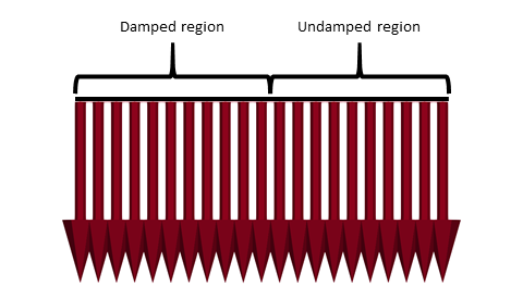
Figure 4: Physical space gradients along the line left half to be restricted.)

Figure 5: Sensitivities along the line when damped region sensitivities are set to zero (left half to be restricted.)
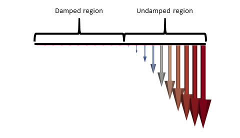
Figure 6: Gradients along the line when damped region is damped using a damping methodology. (left half to be restricted.)
Damping functions
Following damping functions are supported:
Gaussian filter function
$$ A\left(\mathbf{x},\mathbf{x_0},r\right) = \max\left\lbrace 0.0, e^{\frac{-9\left|\mathbf{x}-\mathbf{x_0}\right|^2}{2r^2}}\right\rbrace$$
Linear filter function
$$ A\left(x,x_0,r\right) = \max\left\lbrace 0.0, \frac{r-\left|\mathbf{x}-\mathbf{x_0}\right|}{r}\right\rbrace$$
Constant filter function
$$ A\left(x,x_0,r\right) = 1.0$$
Cosine filter function
$$ A\left(x,x_0,r\right) = \max\left\lbrace 0.0, 1-0.5\left(1-\cos\left(\pi\frac{\left|\mathbf{x}-\mathbf{x_0}\right|}{r}\right)\right)\right\rbrace$$
Quartic filter function
$$ A\left(x,x_0,r\right) = \max\left\lbrace 0.0, \left(\frac{\left|\mathbf{x}-\mathbf{x_0}\right|-r}{r}\right)^4\right\rbrace$$
Vertices for different containers
This vertex morphing and damping are used to compute vertex morphed and constrained gradients of objectives and constraints. The vertex morphing and damping requires always a vertices to compute the smoothen control field in control space.
- In the case physical field is in the
Kratos::NodesContainerType, then it uses nodal locations as the vertices. - In the case physical field is in the
Kratos::ConditionsContainerType, then it uses conditions’ underlying geometry’s center as the vertices. - In the case physical field is in the
Kratos::ElementsContainerType, then it uses elements’ underlying geometry’s center as the vertices.
Damping methodology
Damping factors (i.e. \(\beta_{i, damp}\)) are computed for each \(i^{th}\) vertex in the damping regions as follows. First neighbours of each vertex in the damping region is found using a KDTree search.
$$ \beta_{i, damp} = \min_{x_j \in \Omega_{i, neighbours}} 1.0 - A(x_i, x_j, r) $$
Thereafter, the gradient of the vertex is multiplied by the damping factor to compute the damped sensitivities as shown in the following equation:
$$ \left(\frac{dh}{d\underline{s}}\right)_{i, damped} = \beta_{i, damp}\left(\frac{dh}{d\underline{s}}\right)_i $$
Vertex morphing methodology
Then for each vertex’s (i.e. \(i^{th}\)) neigbhour vertices (i.e. \(j^{th}\)) the weights are computed using filter functions mentioned above (i.e. \(A_{ij}\)). Thereafter, the vertex morphed gradients for each gradient is computed as given in the following equation.
$$ \left(\frac{df}{d\underline{s}}\right)_{i, morphed} = \frac{1}{\sum_{j=1}^N A_{ij}}\sum_{j=1}^{N} A_{ij}\left(\frac{df}{d\underline{s}}\right)_j$$
References
TODO: