Overview
As explained in the home page, the Kratos framework is oriented towards finite element modelling. This is a major advantage when creating standard finite element formulations. In these cases, Kratos will provide most of the tedious code necessary, such as assembling the matrices, solving the system, printing the results in a file, and other task that would probably be more time consuming than transcribing the formulation itself into programming code. The aim of this tutorial is to describe step by step the implementation of a really simple element using as much as possible all these tools provided by Kratos. This way, we’ll only have to create the element, boundary conditions and then tell Kratos that our problem type is a standard FEM. At first the code might seem a little scary but we’ll try to explain the lines as much as possible. Let’s begin!
(it must be noted that the framework is completely flexible and we could create a problem type without even creating an element that does something, for example in edge based formulations)
Basic description of the problem and main tools of Kratos used:
We’ll create the simplest possible finite element formulation. For that purpose we’ll create an application that solves a stationary heat conduction problem in 2D. This is a diffusion only problem with only one degree of freedom (DoF) per node.
\[\nabla · (K\nabla\Phi) = f\]Were \(K\) is the material heat conductivity
In this problem we’re going to use a residualbased formulation. Kratos already has a solver so we won’t have to program it.
As seen in the previous section, our problem consists of a simple rigidity matrix K , that depends only on the geometry and the scalar permittivity (a closer look reveals that is simply the Laplacian matrix multiplied by this scalar). The other components of our problem are boundary conditions, which we will assume fixed or free, and thermal loads.
Components
The rigidity matrix will be calculated element by element, adding the rigidity of each element K to the global matrix. This reveals the first tool needed in our problemtype: an element.
For the Dirichlet conditions, since we’re using a residual-based calculation we’ll have to multiply our boundary conditions by the K matrix. This can be done both element-wise once we have K or at the end of the problem. We chose to do it element-wise.
Finally, for the nodal thermal loads we have to add them node by node and add it to the right hand side vector of the system of equations (RHS). To do so we’ll use a tool in Kratos called Condition.
As you can see, we now have our main application components:
- An element (loop in elements, including K and Dirichlet conditions)
- A condition (loop in nodes)
Residual-based builder and solver
What is missing is a tool to assemble all these components. We could do it “by hand”, but it is much simpler if we just use a builder and solver. Kratos include a residual-based builder and solver. This way we only have to declare in our problem-type that we’ll be using this tool and which are the elements and conditions. And that’s it. We won’t even need to tell the builder to loop the nodes or elements, just declaring them and then initializing the solver is enough and the process will be done.
Of course, to do so we’ll have to respect the structure for both the element and conditions, but this is achieved by simply copying an existing one and modifying it to suit our needs, as will be seen below.
Structure of the problem type and other components
Basic Structure of Conditions and Elements
Elements and Conditions are both classes in C++ that include a series of subroutines required by the builder and solver. They both share the following structure. An element or condition should contain at least this public methods, in pseudo code:
class mycondition

void CalculateLocalSystem
void CalculateRightHandSide
void EquationIdVector
void GetDofList
Python Scripts
At this point we have explained the code needed inside Kratos to solve a Poisson problem. However, no information regarding loading the model or telling Kratos that we want to execute our problem type was given. All these tasks are not compiled in the Kratos, they’re simply executed by python scripts. Some of them will belong to our problem type itself and other will be contained inside the folder of the specific problem to be solved.
The big advantage of using these scripts over compiled code is that changes can be done really quickly, for example changing the tolerance of a solver or even changing boundary conditions. Of course, since it’s interpreted language it will be slower; so it’s better to limit its use to simple, non iterative tasks as much as possible.
In this sense, the python scripts do the following tasks:
- Load Kratos and import our application
- Read the problem data, project parameters and create the model part in Kratos: Mesh, elements, materials, variables, degrees of freedom…
- Define the Builder&Solver used
- Call the solver
- Write a file with the mesh and results
Files needed in our application
Our application will be located inside the applications folder. Each of these subdirectories will contain the specific C++ or python code needed for our application. Note that if you want to use a new strategy or solver, then you have to create other typical customization directories or files such as /custom_strategies, etc…
/Kratos
    /applications
        /PureDiffusionApplication
            /custom_elements
                my_laplacian_element.h and .cpp
            /custom_conditions
                point_source_condition.h and .cpp
            /custom_python
                my_laplacian_application.cpp
            /python_scripts
                static_laplacian_element.py
            my_laplacian_application.h and .cpp
            my_laplacian_application_variables.h and .cpp
            MyLaplacianApplication.py
            CMakeLists.txt
The application will be executed to solve an specific problem defined in few files outside Kratos:
/SpecificProblem
    MainKratos.py
    specific_problem.mdpa
    ProjectParameters.json
Now you should have an idea of the components we will need in our code. So hands at work with C++ and Python.
Sections of this tutorial
Creating our application: MyLaplacianApplication
First of all, we recommend to create a temporary branch. In this way, we could easily revert the changes we make. Just open the terminal and type:
$ git checkout -b test-kratos-for-dummies
To begin with we must create a new application. The How to Create Applications tutorial provide some python scripts to generate a base application. Therefore we’ll navigate to the kratos/python_scripts/application_generator folder and customize the laplacian_application_example.py script. We need to specify the application name, elements and conditions. Note that we have to create a new variable POINT_HEAT_SOURCE, which is not inside the Kratos’s kernel.
# Set the application name and generate Camel, Caps and Low
appNameCamel = "MyLaplacian"

# Fetch the applications directory
debugApp = ApplicationGenerator(appNameCamel)

# Add KratosVariables
debugApp.AddVariables([
    VariableCreator(name='POINT_HEAT_SOURCE', vtype='double'),
])

# Add an element
debugApp.AddElements([
    ElementCreator('MyLaplacianElement')
    .AddDofs(['TEMPERATURE'])
    .AddFlags([])
    .AddClassMemberVariables([])
])

# Add a condition
debugApp.AddConditions([
    ConditionCreator('PointSourceCondition')
    .AddDofs(['TEMPERATURE'])
    .AddFlags([])
])
The python script will create a new application with the basic components. In order to compile the application, we need to add it in the configure.shfile:
add_app ${KRATOS_APP_DIR}/MyLaplacianApplication
Once you’ve followed all the steps and compiled the application, you should be able to import your newly created application, although it is not able to do anything for the moment.
Editing the main files of the application and creating elements and conditions
- Tutorial: Editing the main files
- Tutorial: Creating the Element
- Tutorial: Creating the Conditions
- Tutorial: Creating an Utility (optional). Once you’ve completed these 3/4 first steps and compiled the kratos you have all the c++ code necessary for your application. So compile the Kratos and the rest of the tasks can be managed using python, which has the advantages mentioned above. So now we proceed with the python scripts required.
- Tutorial: Creating the Python Solver file: After you’ve finished these 6 steps your new application is ready. what is left is creating the particular files of our problem.
Creating a first problem to be solved
Despite the GiD interface can both create and launch the files needed to solve a problem, we’ll start by writing ‘by hand’ a very simple example so that we understand the instruction we’re giving KRATOS through the python interface we have just created in the previous step. Actually when you launch an example from the GiD interface of Kratos, this is what is going on behind: First GiD creates a geometry file that Kratos can understand, the .mdpa , and then it executes a python scripts that contains all the instruction for Kratos. Like read the geometry, add degrees of freedom, solve the system, print the results…
So hands at work! We need these two files to launch an example:
- A .mdpa (meaning modelpart) file defining the geometry, material, loads, etc.
- A .json file defining the required project parameters.
- A .py file to tell Kratos what to do with that file.
For our first problem we’ll create a simple, two element problem:

with CONDUCTIVY=10.0, we’ll fix the TEMPERATURE=100.0 in node 1 and we’ll add a POINT_HEAT_SOURCE=5.0 in node 3
with this information, the model part file looks like this:
example.mdpa
Begin ModelPartData
//  nothing here
End ModelPartData


Begin Properties 1
CONDUCTIVITY 10.0 // all the elements of the group 1 (second column in the list of elements) will have this property
End Properties

Begin Nodes
       1        0.0        0.0         0.0     //node number, coord x, cord y, coord z
       2        1.0        0.0         0.0     //node number, coord x, cord y, coord z
       3        1.0        1.0         0.0     //node number, coord x, cord y, coord z
       4        0.0        1.0         0.0     //node number, coord x, cord y, coord z
End Nodes

Begin Elements MyLaplacianElement //here we must write the name of the element that we created
  1 1 1 2 4   //pos1:elem ID ; pos2:elem Property ( = 1 in this case) ; pos3 - pos5: node1-node3
  2 1 3 4 2   //pos1 and pos2 are always id and property. if the elem had 4 nodes, we woud add a 6th column for the last node
End Elements

Begin NodalData TEMPERATURE          //be careful, variables are case sensitive!
1 1 100.0                // pos1 is the node, pos2 (a 1) means that the DOF is fixed, then (position 3) we write the fixed displacement (in this case, temperature)
End NodalData

Begin NodalData POINT_HEAT_SOURCE
3    0    5.0             //fixing it or not does not change anything since it is not a degree of freedom, it's just info that will be used by the condition
End NodalData

Begin Conditions PointSourceCondition
1 1 3     //pos1:condition ID(irrelevant) ; pos2:cond Property ( = 1 in this case) ; pos3:node to apply the condition. if it was a line condition, then we would have 4 numbers instead of 3, just like elements
End Conditions
our ProjectParameters.json file:
ProjectParameters.json
{
	"model_import_settings"        : {
		"input_type"          : "mdpa",
		"input_filename"      : "unknown_name"
	},
	"echo_level"                   : 0,
	"buffer_size"                  : 2,
	"relative_tolerance"           : 1e-6,
	"absolute_tolerance"           : 1e-9,
	"maximum_iterations"           : 20,
	"compute_reactions"            : false,
	"reform_dofs_at_each_step"     : false,
	"calculate_norm_dx"            : true,
	"move_mesh_flag"               : false,
	"linear_solver_settings"       : {
			"solver_type"     : "skyline_lu_factorization"
	}
}
and our python file:
example.py
def Wait():
	input("Press Something")

#including kratos path
import sys
from KratosMultiphysics import *
#import KratosMultiphysics    #we import the KRATOS
import KratosMultiphysics.MyLaplacianApplication as Poisson       #and now our application. note that we can import as many as we need to solve our specific problem


#setting the domain size for the problem to be solved
domain_size = 2  # 2D problem

#defining a model part
model = Model()
model_part = model.CreateModelPart("Main");  #we create a model part

import KratosMultiphysics.MyLaplacianApplication.pure_diffusion_solver as pure_diffusion_solver           #we import the python file that includes the commands that we need
parameter_file = open("ProjectParameters.json",'r')  # we read the ProjectParameters.json file
custom_settings = Parameters(parameter_file.read())

pure_diffusion_solver = pure_diffusion_solver.CreateSolver(model, custom_settings)
pure_diffusion_solver.AddVariables()  #from the static_poisson_solver.py we call the function Addvariables so that the model part we have just created has the needed variables

 # (note that our model part does not have nodes or elements yet)

 #now we proceed to use the GID interface (both to import the infomation inside the .mdpa file and later print the results in a file
gid_mode = GiDPostMode.GiD_PostAscii  #we import the python file that includes the commands that we need
multifile = MultiFileFlag.SingleFile
deformed_mesh_flag = WriteDeformedMeshFlag.WriteUndeformed
write_conditions = WriteConditionsFlag.WriteElementsOnly
gid_io = GidIO("art4", gid_mode,multifile, deformed_mesh_flag, write_conditions)

model_part_io = ModelPartIO("example")          # we set the name of the .mdpa file
model_part_io.ReadModelPart(model_part)         # we load the info from the .mdpa

# we create a mesh for the postprocess
mesh_name = 0.0
gid_io.InitializeMesh( mesh_name )
gid_io.WriteMesh((model_part).GetMesh())
gid_io.FinalizeMesh()

#the buffer size should be set up here after the mesh is read for the first time  (this is important for transcient problems, in this static problem =1 is enough)
model_part.SetBufferSize(1)

# we add the DoFs
pure_diffusion_solver.AddDofs()

# Initialize the solver
pure_diffusion_solver.Initialize()

print ("about to solve!")
pure_diffusion_solver.Solve()
print ("Solved!")

#and we print the results
gid_io.InitializeResults(mesh_name,(model_part).GetMesh())
gid_io.WriteNodalResults(TEMPERATURE,model_part.Nodes,0,0)
gid_io.FinalizeResults()

# since we have already calculated the temp, we can get the mean value
# first the constructor (it could have been called before)
try:
	calc_mean = Poisson.CalculateMeanTemperature(model_part)
    # and we calculate!
	calc_mean.Execute()
except:
	pass
Launching and viewing the postprocess file
Once you have both files, you must open a console, go the directory where you created both files and type:
$ python example.py
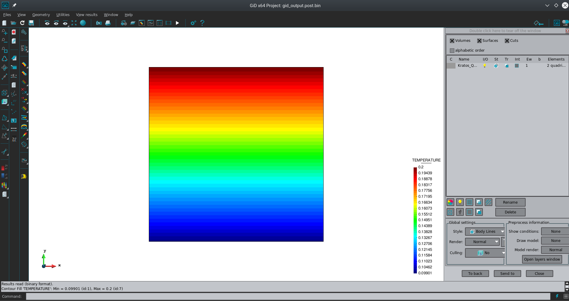
This launches the script you’ve created and several files are created after it has finished. The ones we are interested in are output.res and output.msh (results and mesh respectively). They are ASCII files so you can view them using the text editor you prefer. Alternatively, you can open the .res with GiD to visualize them. The result should look like this:
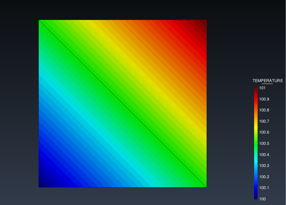
Congratulations!, you have successfully created and launched your first python application.
Using the GiD problemtype
NOTE: There is a new interface in GiD, the interface example is not implemented yet.
Using the GiD interface allows you to manage much more complex geometries. Moreover, you can launch Kratos directly from the (visual) GiD interface, so there’s no longer need to use a console. To do so simply download File:PureDiffusion.gid.zip and unzip it inside the GiD problemtypes folder. The interface is really easy to use so you should have no problems understanding how to use it.