Edit me

Overview

This tutorial introduces one alternative for effectively interacting with a Kratos simulation to modify some of its parameters and observe the effect of such a modification on the results in real-time. Admittedly, this can be achived for any of the simulations available in Kratos, however, it is particularly suitable for fast simulations, like the ones achived by using Reduced Order Models ROM. Therefore, this tutorial focuses on an example using the RomApplication. The Python module vedo is used for the interactive visualization.

Content

What is vedo?

(vedo) is a lightweight and powerful python module for scientific analysis and visualization of 3D objects. It is based on numpy and VTK, with no other dependencies.

Installation

The following section guides the user toward the setting up of the Kratos applications and installation of vedo to run the example case.

This example uses an earlier version of the vedo module. Therefore, please install using the command provided below, and not the one for the latest version of vedo in vedo’s repository.

# installing earlier version of vedo (previously known as vtkplotter)
pip3 install vtkplotter==2020.0.1

Make sure to install the applications required. In this example the RomApplication and the StructuralMechanicsApplication are used. Therefore, add both these application to the Kratos configure file.

Linux:

add_app ${KRATOS_APP_DIR}/StructuralMechanicsApplication
add_app ${KRATOS_APP_DIR}/RomApplication

Windows:

CALL :add_app %KRATOS_APP_DIR%/StructuralMechanicsApplication
CALL :add_app %KRATOS_APP_DIR%/RomApplication

How to use vedo for interacting with the simulation

In this section, a simple example is used to illustrate the approach taken to interactively modify the parameters of a simulation in Kratos. Download the files for this example here .

Problem definition

A static structural example has been chosen for demonstrating the integration of vedo into the simulation. The selected geometry is the Stanford bunny. As can be seen, displacement constraints are being applied to the base and a varying pressure is applied to the face of the bunny. 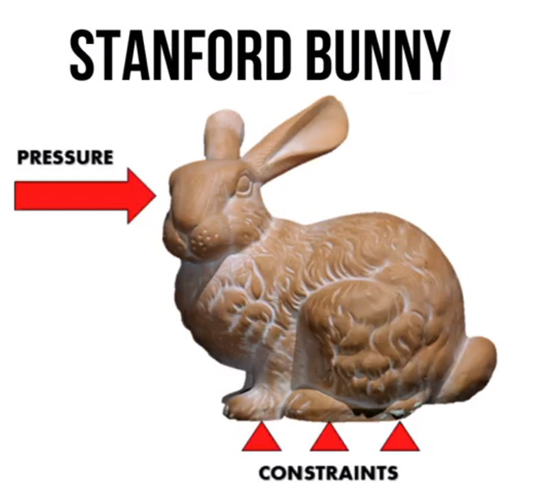bunny

The original model from which this Reduced Order Model was obtained contained 30.000 elements, therefore it was too slow for solving it in real time. On the other hand, the ROM only requires the evaluation of 50 elements to obtain the results.

Integration of vedo

Thanks to the Python interface of Kratos, the vedo module can be used by simply calling it inside a derived class in the original MainKratos.py.

We start now analyzing how vedo is defined inside our code. First of all we observe the import statement (notice vedo’s old version is called vtkplotter):

#Import visualization tool
import vtkplotter

In order to change the magnitude of the load applied, we will use an on-screen slider; for which we define the slider class. Notice that we are going to apply this pressure in MPa, but Kratos is expecting a pressure in Pa, therefore we take into account the 1e6 factor here.

#Slider class
class Slider():
    def __init__(self, InitialValue):
        self.value = InitialValue

    def GenericSlider(self,widget, event):
        value = widget.GetRepresentation().GetValue()*1e6
        self.value = value

Inside a class derived from StructuralMechanicsAnalysisROM and which we have called InteractiveSimulation in this example, we define the Plotter object as an attribute of InteractiveSimulation. Moreover we add to it the slider for modifying the pressure.

self.slider1 = Slider(0)
self.Plot = vtkplotter.Plotter(title="Simulation Results",interactive=False)
self.Plot.addSlider2D(self.slider1.GenericSlider, -200, 400 , value = 0, pos=3, title="Pressure (MPa)")

The method ApplyBoundaryConditions will capture the current position of the slider before each solve step, and will apply the corresponding pressure to the simulation by employing the AssignScalarVariableToConditionsProcess.

def ApplyBoundaryConditions(self):
    super().ApplyBoundaryConditions()
    Pressure = self.slider1.value
    print(f'Pressure is {Pressure} Pa')
    PressureSettings = KratosMultiphysics.Parameters("""
    {
        "model_part_name" : "Structure.COMPUTE_HROM.SurfacePressure3D_Pressure_on_surfaces_Auto4",
        "variable_name"   : "POSITIVE_FACE_PRESSURE",
        "interval"        : [0.0,"End"]
    }
    """
    )
    PressureSettings.AddEmptyValue("value").SetDouble(Pressure)
    AssignScalarVariableToConditionsProcess(self.model, PressureSettings).ExecuteInitializeSolutionStep()

Vedo allows the definition of generic buttons to perform some action on the visualization. For this example, we define 2 buttons: for pausing-continuing and for stoping the simulation.

self.PauseButton = self.Plot.addButton(
    self.PauseButtonFunc,
    pos=(0.9, .9),  # x,y fraction from bottom left corner
    states=["PAUSE", "CONTINUE"],
    c=["w", "w"],
    bc=["b", "g"],  # colors of states
    font="courier",   # arial, courier, times
    size=25,
    bold=True,
    italic=False,
)

self.StopButton = self.Plot.addButton(
    self.StopButtonFunc,
    pos=(0.1, .9),  # x,y fraction from bottom left corner
    states=["STOP"],
    c=["w"],
    bc=["r"],  # colors of states
    font="courier",   # arial, courier, times
    size=25,
    bold=True,
    italic=False,
)

def PauseButtonFunc(self):
    vtkplotter.printc(self.PauseButton.status(), box="_", dim=True)
    if self.PauseButton.status() == "PAUSE":
        self.Plot.interactive = True
    else:
        self.Plot.interactive = False
    self.PauseButton.switch() # change to next status


def StopButtonFunc(self):
    vtkplotter.printc(self.StopButton.status(), box="_", dim=True)
    if self.StopButton.status() == "STOP":
        self.Finalize()
        self.Continue = False

Finally, the results to plot are retrived from the vtk_output folder after each solve step by calling the FinalizeSolutionStep method. In this method a mesh object of vedo has been defined (stored in self.a), and to this vedo mesh object, the new displacements are added in order to visualize the deformed configuration.

def FinalizeSolutionStep(self):
    super().FinalizeSolutionStep()
    if self.timestep>1.5:
        if self.timestep==2:
            self.a = vtkplotter.load(f'./vtk_output/VISUALIZE_HROM_0_{self.timestep}.vtk')
            displs = self.a.getPointArray("DISPLACEMENT")

        if self.timestep>2:
            b = vtkplotter.load(f'./vtk_output/VISUALIZE_HROM_0_{self.timestep}.vtk')
            newpoints = b.points()
            displs = b.getPointArray("DISPLACEMENT")
            self.a.points(newpoints+displs)

        self.a.pointColors(vtkplotter.mag(displs), cmap='jet').addScalarBar(vmin = 0, vmax = 0.009)
        self.a.show(axes=1, viewup='z')
    self.timestep +=1

Changing boundary conditions in real time

We can proceed to run the example with the usual command

python3 MainKratos.py

Then, the terminal will show the usual output of a Kratos simulation while a vedo window will appear showing the real-time solution. Grab and hold the slider to modify the load applied on the face of the Stanford Bunny. You will observe the corresponding deformation immediately.

Pressing the PAUSE button will interrupt the loop over this static simulation. After pressing PAUSE, the button will display CONTINUE. Press CONTINUE again to carry on with the simulation loop (You might need to press the spacebar after pressing CONTINUE).

Press the STOP button to call the Finalize method and finish the simulation.

demo

How to interact with a simulation to visualize real time results