Sources. Thesis §4.4.4 (pp. 129–130: penetration definition, consistent gap, Figs. 4.34, 4.35), Appendix E.1 (p. 339, Algorithm 8 “Consistent gap computation”), §4.3.3.4.2 (mortar operators); code:
custom_processes/normal_gap_process.{h,cpp},custom_processes/base_contact_search_process.cpp,custom_processes/simple_contact_search_process.cpp,custom_processes/advanced_contact_search_process.{h,cpp},custom_utilities/mortar_explicit_contribution_utilities.cpp,custom_utilities/contact_utilities.cpp,custom_processes/compute_dynamic_factor_process.cpp,custom_strategies/custom_strategies/residualbased_newton_raphson_contact_strategy.h,custom_strategies/custom_convergencecriterias/base_mortar_criteria.h,python_scripts/search_base_process.py, Kratos corekratos/processes/simple_mortar_mapper_process.h,kratos/utilities/exact_mortar_segmentation_utility.{h,cpp}; teststests/cpp_tests/processes/test_weighted_gap.cpp.
The search described in Search pipeline and bounding volumes yields candidate pairs of slave and master conditions. Whether a candidate is kept, and whether the slave nodes enter the active set, depends on how far the surfaces are from each other. This page explains the two gap measures used by the application, how they are computed and how they are compared with the thresholds. Notation follows the thesis: superscript \(1\) is the slave side, \(2\) the master side, \(\mathbf{n}\) the slave normal, \(g_n\) the (consistent) normal gap, \(\tilde{g}_n\) the weighted gap, \(\mathbf{D}\) and \(\mathbf{M}\) the mortar operators, \(\Phi_j\) the dual shape functions and \(N_k\) the standard ones.
Penetration definition (thesis §4.4.4)
In an implicit analysis potential contact pairs must be created before penetration happens, i.e. slave nodes approaching a master surface must be detected at a certain distance, the maximal detection distance (MDD). The MDD is a significant parameter of the detection procedure: it should be as small as possible, to avoid unnecessary pairs, but large enough to capture the contact that will develop during the step. The thesis defines it automatically from the element size \(h\) (in the code: NODAL_H, computed by FindNodalHProcess in SearchBaseProcess.ExecuteInitialize, scaled by active_check_factor). Once the MDD is defined, the penetration (or gap) of each node has to be estimated in order to be compared with it.
Conventional penetration estimates (segment intersection, volume intersection, node in volume, node under surface, ray tracing; thesis Fig. 4.25) are usually uncoupled from the contact formulation. The application instead uses a consistent estimate: the very same mortar formulation that defines the weighted gap in the conditions is used to compute a nodal gap during the search. The consistent gap is obtained by mapping the coordinates of one surface onto the other with the mortar mapper (Appendix E) and evaluating node by node
$$ g_n = - \mathbf{n} \cdot \left( \mathbf{x}_1 - \chi_h \, \mathbf{x}_2 \right), $$
where \(\chi_h \mathbf{x}_2\) are the master coordinates mapped onto the slave node. This value has length units and can be compared with a reference length, unlike the weighted gap. As the thesis notes, the consistent gap coincides with the weighted gap divided by the mortar integration area of the node (Fig. 4.34): the NODAL_AREA \(A_j = D_{jj}\).
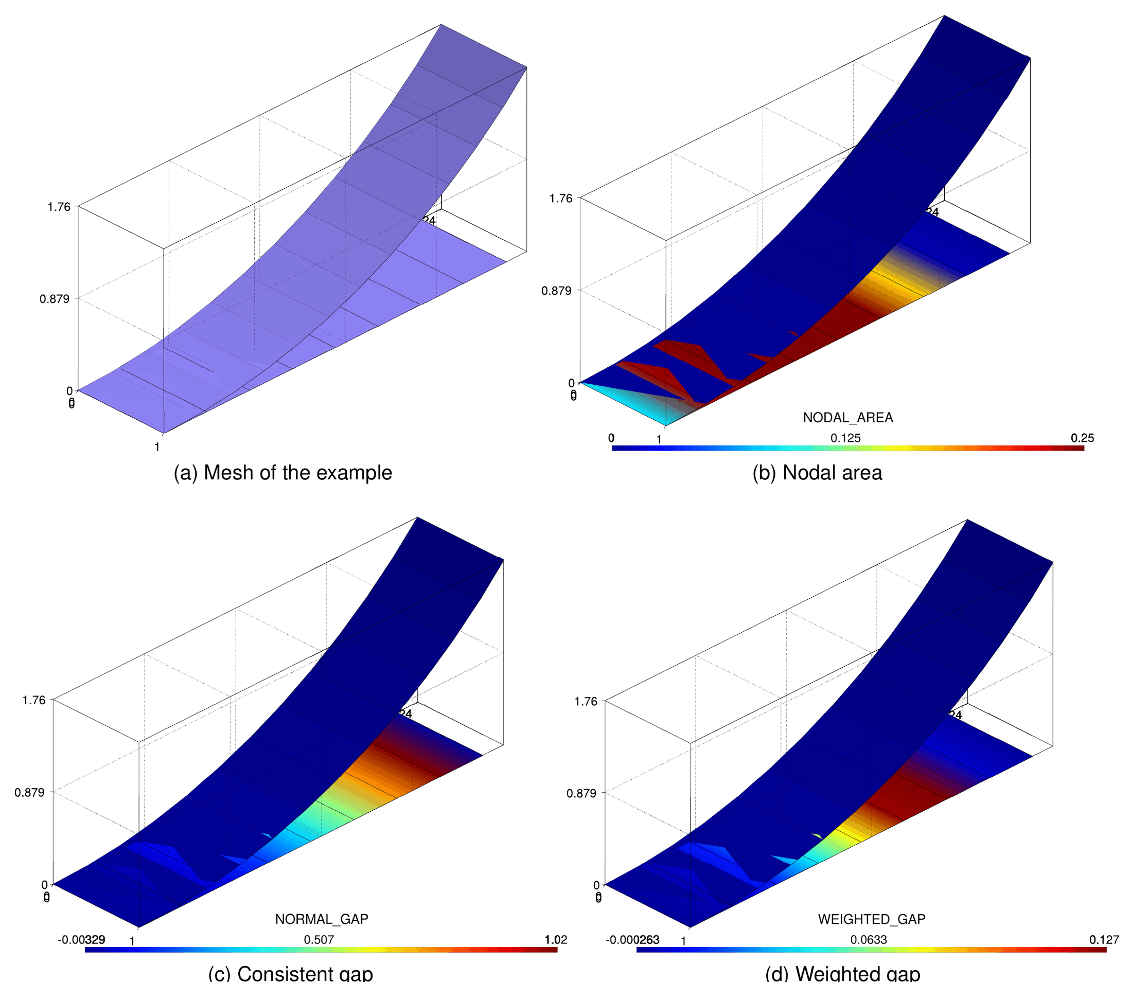
Figure: Consistent gap example, circular surface vs. plane: (a) mesh, (b) nodal area, (c) consistent gap NORMAL_GAP, (d) weighted gap WEIGHTED_GAP. Dividing (d) by (b) recovers (c), which coincides with the analytical height to the circle (thesis Fig. 4.34).
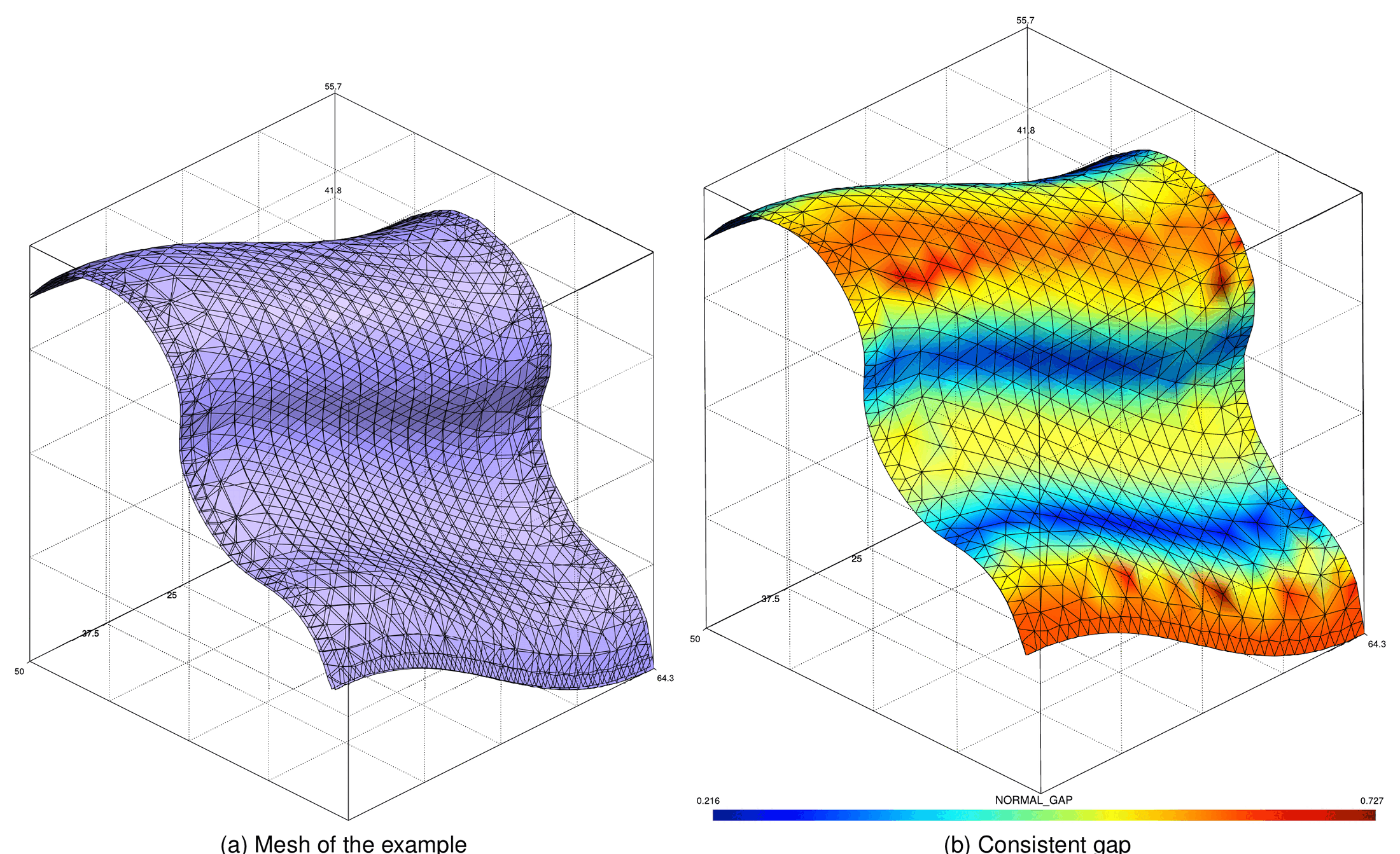
Figure: Consistent gap example on the double-curvature surfaces used to test the mortar mapper: (a) mesh, (b) consistent gap. The gap follows the curvature "parallel lines"; peaks appear at the nodes of the coarse regions (thesis Fig. 4.35).
The two gap measures
Consistent nodal gap: NORMAL_GAP (thesis Algorithm 8)
The procedure is Algorithm 8 of the thesis (Appendix E.1):
Algorithm 8  Consistent gap computation
 1: procedure CONSISTENT GAP COMPUTATION
 2:     Reset auxiliary values for the nodal coordinates on the origin mesh  x_aux
 3:     for all node ∈ OriginMesh_nodes do
 4:         x_aux = x_node
 5:     for all node ∈ DestinationMesh_nodes do
 6:         x_aux = 0
 7:     Map x_aux from OriginMesh_nodes → DestinationMesh_nodes           (mortar mapper)
 8:     for all node ∈ DestinationMesh_nodes do
 9:         From node get the normal (n)
10:         g_consistent = − n · (x_node − x_aux)
It is implemented by NormalGapProcess<TDim, TNumNodes, TNumNodesMaster> (custom_processes/normal_gap_process.{h,cpp}), constructed with the MasterSubModelPart<N> and SlaveSubModelPart<N> model parts and a boolean SearchOrientation (true for the normal search, false for an inverted search):
AUXILIAR_COORDINATESof the master (origin) nodes are set to their coordinates and those of the slave (destination) nodes to zero (lines 2–6). In the inverted case the roles and theMASTER/SLAVEflags are swapped (SwitchFlagNodes).- A
SimpleMortarMapperProcess<TDim, TNumNodes, Variable<array_1d<double,3>>, TNumNodesMaster>mapsAUXILIAR_COORDINATESfrom master to slave (line 7) with the parameters{"distance_threshold": ProcessInfo[DISTANCE_THRESHOLD], "update_interface": false, "remove_isolated_conditions": true, "origin_variable_historical": false, "destination_variable_historical": false, "zero_tolerance_factor": ProcessInfo[ZERO_TOLERANCE_FACTOR], "consider_tessellation": Properties[CONSIDER_TESSELLATION]}. The mapper uses the dual Lagrange multiplier mortar projection described in Mortar integration and dual Lagrange multipliers, so it shares the exact integration (ExactMortarIntegrationUtility) with the contact conditions. ComputeNormalGapevaluates lines 8–10 for the slave nodes with the nodalNORMALand stores the result in the non-historical variableNORMAL_GAP; nodes on which nothing was mapped (AUXILIAR_COORDINATESstill zero, i.e. no master found withinDISTANCE_THRESHOLD) keep the previous value, and master nodes getNORMAL_GAP = 0.
BaseContactSearchProcess::ComputeMappedGap runs this process from CheckPairing, after initializing NORMAL_GAP of the whole ContactSub<N> to \(10^{12}\) so that unmapped nodes are recognized as far away. Sign convention: NORMAL_GAP is negative when the slave node penetrates the master surface and positive when there is a gap.
Weighted gap: WEIGHTED_GAP
The weighted gap is the quantity that actually enters the contact conditions (see Frictionless contact). For slave node \(j\) it is the dual-weighted integral of the gap over the slave surface, which in discrete form reads
$$ \tilde{g}_{n,j} = - \mathbf{n}_j \cdot \left( \mathbf{D} \, \mathbf{x}_1 - \mathbf{M} \, \mathbf{x}_2 \right)_j , \qquad D_{jk} = \int_{\Gamma_c^1} \Phi_j N^1_k \, d\Gamma, \quad M_{jl} = \int_{\Gamma_c^1} \Phi_j \left( N^2_l \circ \chi_h \right) d\Gamma . $$
In the code it is assembled explicitly (no system solve) by MortarExplicitContributionUtilities::AddExplicitContributionOfMortarCondition (frictionless) and AddExplicitContributionOfMortarFrictionalCondition (adds WEIGHTED_SLIP), called from the AddExplicitContribution method of every paired mortar condition. For each condition of ComputingContact:
- an
ExactMortarIntegrationUtilityis created with theINTEGRATION_ORDER_CONTACTof the properties,ProcessInfo[DISTANCE_THRESHOLD](default \(10^{24}\)),ProcessInfo[ZERO_TOLERANCE_FACTOR](default \(1\)) andCONSIDER_TESSELLATION, and the master is clipped against the slave (GetExactIntegration); - if the clipping is non-empty and the integrated area exceeds \(10^{-5}\) of the slave area, the mortar operators are computed and
NODAL_AREAreceives the diagonal \(D_{jj}\) (AtomicAdd); - the rows of \(\mathbf{D}\mathbf{x}_1 - \mathbf{M}\mathbf{x}_2\) are dotted with the negative nodal normal and accumulated into the historical variable
WEIGHTED_GAPof the slave nodes; in the frictional case the tangential part of the time derivative of the same expression, computed with the previous mortar operators (objective slip) or with the displacement increments (non-objective slip, conditions flaggedMODIFIED), is accumulated intoWEIGHTED_SLIP.
Because the contributions of all the paired conditions sharing a slave node are summed, WEIGHTED_GAP must be reset to zero before every evaluation. ContactUtilities::ComputeExplicitContributionConditions(rModelPart) loops over the conditions of ComputingContact and calls AddExplicitContribution; it is invoked at four points of the solution process:
| Where | When | Purpose |
|---|---|---|
BaseContactSearchProcess::ComputeWeightedReaction |
End of every search (UpdateMortarConditions, CheckPairing) |
Provide WEIGHTED_GAP/WEIGHTED_SLIP (or the mesh-tying residuals WEIGHTED_SCALAR_RESIDUAL, WEIGHTED_VECTOR_RESIDUAL) for the activation criteria |
ResidualBasedNewtonRaphsonContactStrategy::Predict |
Start of the step, before the first iteration | Gap of the predicted configuration (see below) |
BaseMortarConvergenceCriteria::PreCriteria |
Every non-linear iteration when ADAPT_PENALTY is on or VELOCITY exists |
Gap needed by the adaptive penalty and the dynamic factor |
BaseMortarConvergenceCriteria::PostCriteria |
Every non-linear iteration | Saves the current gap in buffer position 1, recomputes it in position 0; used by the active-set check and the frictional criteria |
The DISTANCE_THRESHOLD and ZERO_TOLERANCE_FACTOR values are consumed inside ExactMortarIntegrationUtility: a master whose projected distance exceeds mDistanceThreshold is skipped entirely, and mZeroToleranceFactor * ZeroTolerance is the geometric tolerance of the inside/clipping checks (CheckInside). zero_tolerance_factor is exposed in the contact process settings (1.0 for ALM/penalty, 1.0e2 for the MPC process) and copied to ProcessInfo[ZERO_TOLERANCE_FACTOR] by SearchBaseProcess._initialize_process_info.
The relation between the two measures is the one stated in the thesis and used throughout the code: \(g_{n,j} \approx \tilde{g}_{n,j} / A_j\). ComputeDynamicFactorProcess writes exactly this ratio into NORMAL_GAP of the active slave nodes, and the advanced activation compares WEIGHTED_GAP / NODAL_AREA with the same length thresholds as NORMAL_GAP.
check_gap modes
The check_gap key of search_parameters selects how the candidates delivered by the broad/narrow phase are turned into pairs and which nodes are activated (BaseContactSearchProcess::ConvertCheckGap, enum CheckGap):
| JSON value | CheckGap |
Pair creation | Activation |
|---|---|---|---|
"NoCheck" / "no_check" |
NoCheck = 0 |
Every candidate that passes the orientation filter becomes a paired condition immediately (AddPotentialPairing → AddPairing) |
All nodes of every paired slave are set ACTIVE |
"DirectCheck" / "direct_check" |
DirectCheck = 1 |
The candidate is paired if at least one slave node projects inside the master closer than NODAL_H * ACTIVE_CHECK_FACTOR |
The nodes satisfying the projection test are set ACTIVE; nodes already ACTIVE count as potential contact |
"MappingCheck" / "mapping_check" (default; the Python default "check_mapping" also resolves here) |
MappingCheck = 2 |
Candidate ids are stored in the slave INDEX_MAP; after NormalGapProcess, CreateAuxiliaryConditions creates a paired condition for every stored id |
ComputeActiveInactiveNodes compares NORMAL_GAP (and WEIGHTED_GAP / NODAL_AREA) with the thresholds |
The direct check (AddPotentialPairing) projects each inactive slave node onto the master geometry with GeometricalProjectionUtilities::FastProjectDirection, first along the nodal normal (or the slave condition normal if the nodal one is zero) and then along the reversed master normal; the node is activated if the projection distance is at most NODAL_H * ACTIVE_CHECK_FACTOR and the projected point is inside the master (IsInside with ZeroTolerance). It does not require the mapper and is therefore cheaper, but it gives a nodal, not a consistent, estimate of the gap and is not compatible with the advanced activation, which needs NORMAL_GAP.
With NoCheck and DirectCheck the weighted gap is still integrated at the end of the search (ComputeWeightedReaction), so the conditions start the step with a meaningful WEIGHTED_GAP.
Activation thresholds
The quantities involved in the decision “is this slave node active?” are:
| Quantity | Where it lives | Value / default | Set by | Used by |
|---|---|---|---|---|
ACTIVE_CHECK_FACTOR |
ProcessInfo and contact Properties |
search_parameters["active_check_factor"] (default 0.01, multiplied by \(h_{max}/h_{min}\) when adapt_search) |
SearchBaseProcess._initialize_process_info, _initialize_search_values |
AddPotentialPairing (times NODAL_H), AdvancedContactSearchProcess::ComputeActiveInactiveNodes (times DISTANCE_THRESHOLD) |
DISTANCE_THRESHOLD |
ProcessInfo |
1.0e24 at initialization; max(mean NODAL_H slave, mean NODAL_H master) after every advanced search |
SearchBaseProcess._initialize_search_values, AdvancedContactSearchProcess::CheckPairing |
NormalGapProcess (mapper), ExactMortarIntegrationUtility (integration cut-off), advanced activation |
ZERO_TOLERANCE_FACTOR |
ProcessInfo |
zero_tolerance_factor (1.0; 1.0e2 for MPC) |
SearchBaseProcess._initialize_process_info |
Geometric tolerance of the mortar integration and the mapper |
GapThreshold |
static constexpr |
2.0e-3 in BaseContactSearchProcess, 2.0e-4 in AdvancedContactSearchProcess |
compile time | Base criterion (times NODAL_H) and consider_gap_threshold |
NODAL_H |
Historical nodal variable | Mesh size around the node | FindNodalHProcess |
Both criteria |
NODAL_AREA |
Non-historical nodal variable | \(A_j = D_{jj}\) | Explicit contribution | Normalization of WEIGHTED_GAP, LM initial guess |
Simple activation (SimpleContactSearchProcess, base ComputeActiveInactiveNodes): a slave node is active if
$$ g_{n,j} \lt 2\cdot 10^{-3} \, h_j , $$
otherwise it is deactivated. On activation with penetration (\(g_{n,j} \lt 0\)) the multiplier is initialized with the penalty guess \(\lambda_j = \dfrac{\varepsilon_j}{k} A_j g_{n,j}\) along the normal (VECTOR_LAGRANGE_MULTIPLIER, SCALAR_LAGRANGE_MULTIPLIER or LAGRANGE_MULTIPLIER_CONTACT_PRESSURE), with \(\varepsilon_j\) the nodal INITIAL_PENALTY (or the global one) and \(k\) the SCALE_FACTOR.
Advanced activation (AdvancedContactSearchProcess::ComputeActiveInactiveNodes), in pseudo-code:
L_ref = DISTANCE_THRESHOLD * ACTIVE_CHECK_FACTOR
if predict_correct_lagrange_multiplier:  (a, b) = linear regression of λ_n over g̃_n on the active nodes
for all slave nodes j:
    L = L_ref
    weighted_check = ACTIVE(j) and ( g̃_n,j / A_j < L )
    if static_check_movement and g̃_n,j − g̃_n,j(previous step) > −1e-3 |g̃_n,j|:      # gap not closing
        if consider_gap_threshold and L < GapThreshold (2e-4):  L = GapThreshold
    if NORMAL_GAP(j) < L  or  weighted_check:
        if predict_correct_lagrange_multiplier: SetActiveNodeWithRegression(j, a, b)
        else:                                   SetActiveNode(j)
    else:
        SetInactiveNode(j)
SetActiveNode sets ACTIVE and MARKER (so that a later SetInactiveNode in the same search cannot undo it) and, in frictional problems, SLIP = true for nodes with zero FRICTION_COEFFICIENT or when pure_slip, SLIP = false otherwise if undefined. SetInactiveNode clears ACTIVE, zeroes the multiplier of the node (VECTOR_LAGRANGE_MULTIPLIER, SCALAR_LAGRANGE_MULTIPLIER or LAGRANGE_MULTIPLIER_CONTACT_PRESSURE according to TypeSolution) and sets NORMAL_GAP = 0 so that the post-process shows something meaningful. Note that the activation decided by the search is only the initial guess of the step: the semi-smooth Newton active-set strategy of Strategies and convergence criteria updates the ACTIVE flags at every iteration from the augmented pressure.
Lagrange multiplier prediction and correction (predict_correct_lagrange_multiplier: true). ComputeLinearRegressionGapPressure fits \(\lambda_n = a + b \, \tilde{g}_n\) over the currently active nodes (with \(\lambda_n\) either LAGRANGE_MULTIPLIER_CONTACT_PRESSURE or \(\boldsymbol{\lambda} \cdot \mathbf{n}\)). Newly activated nodes receive the predicted pressure \(\min(a + b \tilde{g}_{n,j}, 0)\) (Predict*MortarLM), nodes that stay active are corrected with the same formula (Correct*MortarLM); one implementation exists per TypeSolution (Scalar, Components, ALMFrictionless, ALMFrictionlessComponents, ALMFrictional). This is meant to shorten the first iterations of steps in which the contact area grows.
Gap history, Predict() and the dynamic factor
WEIGHTED_GAP is a historical variable and its buffer is used as a one-step memory of the gap:
BaseMortarConvergenceCriteria::PostCriteriacopiesWEIGHTED_GAPinto buffer position 1 before recomputing it;static_check_movementin the advanced activation andComputeDynamicFactorProcessread the previous value from there.ResidualBasedNewtonRaphsonContactStrategy::Predictdoes not call the base predictor. It zeroesWEIGHTED_GAP(andWEIGHTED_SLIPfor frictional problems) on theContactnodes, recomputes the explicit contribution with the current geometry and then advances the nodal coordinates by the displacement of the step (DISPLACEMENTat step 1,DISPLACEMENT − DISPLACEMENT(1)afterwards), so that the first iteration works on the predicted configuration.ComputeDynamicFactorProcess(executed inPreCriteriawhen the problem is dynamic andcompute_dynamic_factoris on in the convergence criterion, or directly byExplicitPenaltyContactProcess) computes, for every active slave node, \(g_n = \tilde{g}_n / A\) (stored inNORMAL_GAP) and its previous value, and when the node passes from gap to penetration sets
$$ \text{DYNAMIC\_FACTOR} = \min\!\left( 1, \ \frac{\vert g_n \vert}{\vert g_n - g_n^{prev} \vert} \right), $$
i.e. the fraction of the step during which the node was actually in contact. The nodal DYNAMIC_FACTOR multiplies the penalty term of the generated ALM conditions (DynamicFactor vector in CalculateLocalLHS/RHS) and is initialized to one by ALMFastInit. The same process also adapts the nodal INITIAL_PENALTY with a logistic factor of the penetration when MAX_GAP_THRESHOLD is positive (advance_explicit_parameters: max_gap_threshold, max_gap_factor).
Weighted-gap unit tests as executable definitions
tests/cpp_tests/processes/test_weighted_gap.cpp builds small master/slave meshes, pairs every slave with every master into ALMFrictionalMortarContactCondition3D4N (or 2D2N) conditions, and compares the explicitly integrated WEIGHTED_GAP/WEIGHTED_SLIP with independent references. The reference gap is exactly Algorithm 8 applied by hand: AUXILIAR_COORDINATES mapped with SimpleMortarMapperProcess<3, 4, Variable<array_1d<double,3>>> and NORMAL_GAP = −n · (x − x_aux); NODAL_AREA is obtained from a preliminary explicit contribution into NODAL_VOLUME.
| Test | Geometry (helper) | Assertion (tolerance \(10^{-4}\) relative) |
|---|---|---|
WeightedGap1 |
Plane vs. cylinder, 8 divisions, radius 6, angle \(\pi/6\) (CreateNewProblem3D) |
\(\tilde{g}_n / A_j = g_n\) (NORMAL_GAP from the mapper) on every slave node with non-zero weighted gap |
WeightedGap2 |
Same, STEP = 1 |
Same as 1 and WEIGHTED_SLIP = 0 |
WeightedGap3, WeightedGap3b |
Two parallel planes, master shifted by \(\Delta x = 0.1\) (SimplestCreateNewProblem3D, SimpleCreateNewProblem3DGapGap) |
Objective slip: WEIGHTED_SLIP \(/ A_j\) equals \(-\Delta x\) in the shift direction |
WeightedGap4, WeightedGap4b |
Same, conditions flagged MODIFIED |
Non-objective slip gives the same \(-\Delta x\) |
WeightedGap5 |
Plane vs. cylinder with master shift | Objective slip vector equals the imposed shift |
WeightedGap6, WeightedGap7 |
Plane vs. cylinder with master shift | Non-objective slip on the nodes whose gap matches the reference |
WeightedGap8, WeightedGap9 |
2D lines (CreateNewProblem2D), ALMFrictionalMortarContactCondition2D2N |
Weighted slip in 2D, objective and non-objective |
These tests are the executable definition of the two gap measures: the weighted gap normalized by the nodal area must reproduce the consistent gap of the mortar mapper to \(10^{-4}\), which is the statement of Fig. 4.34 in test form. The search-level tests (SearchProcessKDTree*, SearchProcessOctree in test_search_process.cpp) exercise the MappingCheck path end to end, and tests/test_dynamic_search.py checks NORMAL_GAP after a dynamic search against reference JSON files.
Notes and limitations
NORMAL_GAPis a non-historical variable: it is available for post-processing (clear_inactive_for_postzeroes it on inactive nodes) but it is not the quantity used inside the contact conditions, which work withWEIGHTED_GAP.DirectCheckcannot be combined with the advanced activation criteria; useMappingCheck(default) wheneversimple_searchisfalse.- The base
GapThreshold(2.0e-3) and the advanced one (2.0e-4) are compile-time constants; the user-level knob isactive_check_factor. - Nodes without any master within
DISTANCE_THRESHOLDkeepNORMAL_GAP = 1.0e12during the check and are therefore deactivated; if the threshold is too small (very coarse master mesh) the contact may be missed, in which casesearch_factorandactive_check_factorshould be increased oradapt_searchenabled. Predict()moves the nodal coordinates with the step displacement but the geometry used by the explicit contribution is the one before the move; the first Newton iteration recomputes the gap inPostCriteria.
Thesis figures © Vicente Mataix Ferrándiz, PhD thesis “Innovative mathematical and numerical models for studying the deformation of shells during industrial forming processes with the Finite Element Method”, UPC 2020, reproduced by the author. Figures marked “inspired by” are the author’s redrawings of the cited sources.