Sources. Thesis §4.5.4.1.1 (2D plane–sphere Hertz benchmark, Table 4.7, Figs. 4.49–4.51); repository test case
tests/ALM_frictionless_contact_test_2D/hertz_simple_test_parameters.json(ALMHertzSimpleTestContact, validation suite); the output below was produced with the compiled application while writing this page.
The problem
An elastic half-cylinder (radius \(R = 8\), \(E_1 = 200\), \(\nu_1 = 0.3\), plane strain) is pressed onto a much stiffer plate (\(E_2 = 2\times10^{12}\), \(\nu_2 = 0.3\)) by a uniform pressure \(p(t) = 0.2\,t\) applied on its flat top face, in two steps up to \(t \approx 1\). This is the classical Hertz problem: the contact half-width \(a\) and the maximum pressure \(p_{max}\) have closed-form expressions, which is why the thesis uses it (in 2D and 3D, frictionless and frictional) to validate the formulation.
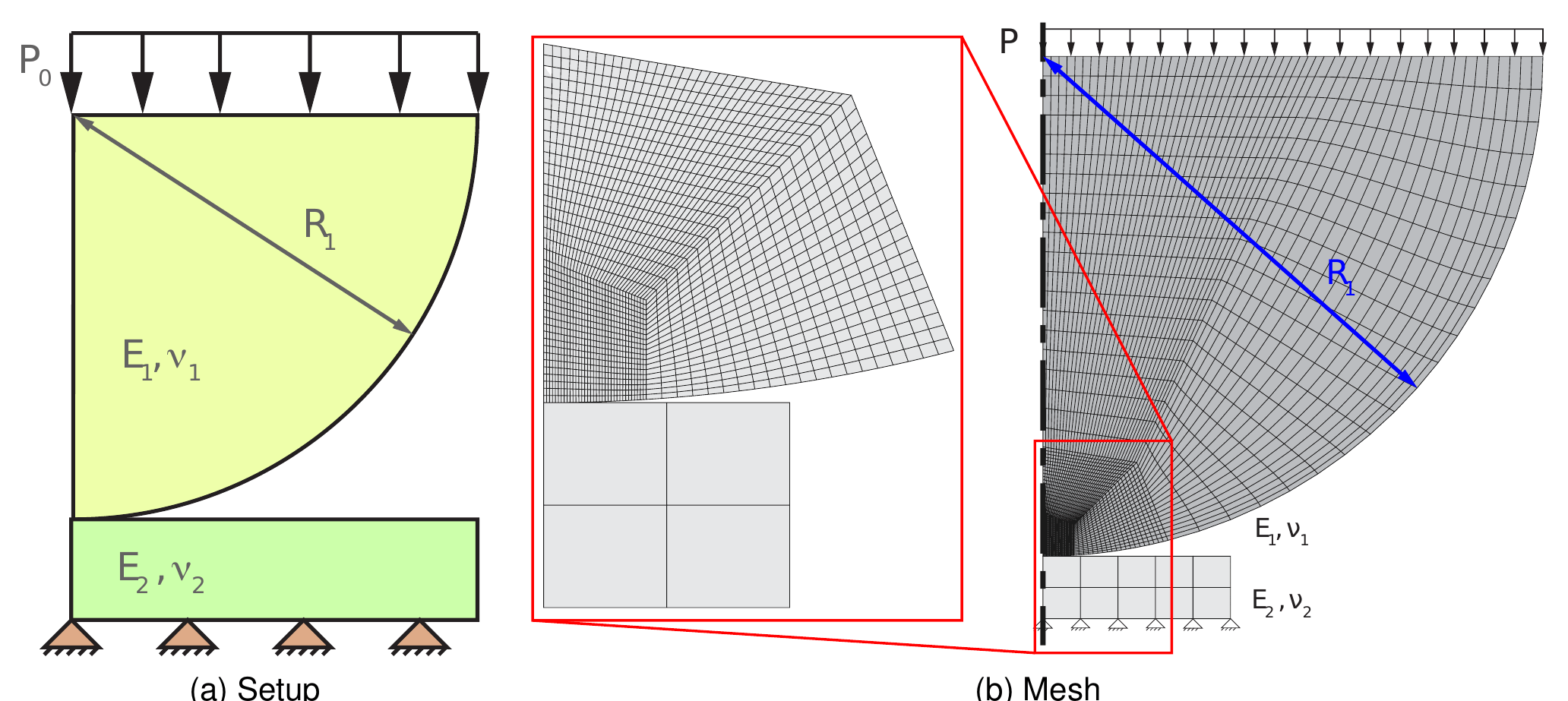
Figure: setup and mesh of the 2D sphere–plane Hertz benchmark (thesis Fig. 4.49).
For a cylinder of radius \(R\) pressed against a plane by a force per unit thickness \(P\) (plane strain), with \(1/E^* = (1-\nu_1^2)/E_1 + (1-\nu_2^2)/E_2\),
$$ a = \sqrt{\frac{4 P R}{\pi E^*}}, \qquad p_{max} = \frac{2P}{\pi a}, \qquad p(x) = p_{max}\sqrt{1 - \left(\frac{x}{a}\right)^2}. $$
Files
Copy the two data files of the test case into a working folder and add the two files written below:
hertz/
├── hertz_simple_test.mdpa            # mesh (3556 nodes, 3400 quadrilaterals), from tests/ALM_frictionless_contact_test_2D/
├── hertz_simple_test_materials.json  # materials, from the same folder
├── ProjectParameters.json            # written below
└── MainKratos.py                     # written below
The mesh defines the sub-model-parts the JSON refers to:
| Sub-model-part | Content | Role |
|---|---|---|
Parts_parts_hemisphere |
SmallDisplacementElement2D4N of the half-cylinder |
deformable body, master side of the contact (assume_master_slave) |
Parts_parts_plate |
SmallDisplacementElement2D4N of the plate |
quasi-rigid body, fully fixed |
LineLoad2D_bc_pressure |
LineLoadCondition2D2N on the flat top of the cylinder |
loaded face (pressure) and horizontally constrained |
DISPLACEMENT_bc_fix |
nodes of the plate base | (fixed through Parts_parts_plate) |
Contact_Part |
the conditions of both contacting surfaces | the interface handed to the contact process |
Note the two ingredients every contact mesh needs: a sub-model-part holding the conditions of all potentially contacting surfaces (Contact_Part), and the possibility to tell which body is master (Parts_parts_hemisphere). Everything else (search, pairing, normals) is done by the application.
hertz_simple_test_materials.json
{
    "properties": [{
        "model_part_name": "Structure.Parts_parts_hemisphere",
        "properties_id": 1,
        "Material": {
            "name": "Material",
            "constitutive_law": { "name": "LinearElasticPlaneStrain2DLaw" },
            "Variables": { "YOUNG_MODULUS": 2.0e2, "DENSITY": 7.85e3, "POISSON_RATIO": 0.3, "THICKNESS": 1.0 },
            "Tables": {}
        }
    },{
        "model_part_name": "Structure.Parts_parts_plate",
        "properties_id": 2,
        "Material": {
            "name": "Material",
            "constitutive_law": { "name": "LinearElasticPlaneStrain2DLaw" },
            "Variables": { "YOUNG_MODULUS": 2.0e12, "DENSITY": 7.85e3, "POISSON_RATIO": 0.3, "THICKNESS": 1.0 },
            "Tables": {}
        }
    }]
}
ProjectParameters.json
The file is the standard structural one plus the two contact blocks highlighted in the comments (contact_settings in the solver, contact_process_list in the processes):
{
    "problem_data"     : {
        "problem_name"  : "hertz_simple_test",
        "parallel_type" : "OpenMP",
        "start_time"    : 0.0,
        "end_time"      : 1.0,
        "echo_level"    : 0
    },
    "solver_settings"  : {
        "model_part_name"                 : "Structure",
        "domain_size"                     : 2,
        "solver_type"                     : "Static",
        "echo_level"                      : 0,
        "analysis_type"                   : "non_linear",
        "model_import_settings"           : {
            "input_type"     : "mdpa",
            "input_filename" : "hertz_simple_test"
        },
        "material_import_settings"        : {
            "materials_filename" : "hertz_simple_test_materials.json"
        },
        "contact_settings"                : {                 // <-- turns the structural solver into a contact solver
            "mortar_type" : "ALMContactFrictionless"
        },
        "time_stepping"                   : {
            "time_step" : 0.5005
        },
        "convergence_criterion"           : "contact_residual_criterion",   // <-- contact-aware criterion
        "displacement_relative_tolerance" : 1.0e-4,
        "displacement_absolute_tolerance" : 1.0e-9,
        "residual_relative_tolerance"     : 1.0e-4,
        "residual_absolute_tolerance"     : 1.0e-9,
        "max_iteration"                   : 20,
        "linear_solver_settings"          : {
            "solver_type" : "skyline_lu_factorization"
        }
    },
    "processes"        : {
        "constraints_process_list" : [{
            "python_module" : "assign_vector_variable_process",
            "kratos_module" : "KratosMultiphysics",
            "process_name"  : "AssignVectorVariableProcess",
            "Parameters"    : {
                "model_part_name" : "Structure.Parts_parts_plate",
                "variable_name"   : "DISPLACEMENT",
                "constrained"     : [true, true, true],
                "value"           : [0.0, 0.0, 0.0]
            }
        },{
            "python_module" : "assign_vector_variable_process",
            "kratos_module" : "KratosMultiphysics",
            "process_name"  : "AssignVectorVariableProcess",
            "Parameters"    : {
                "model_part_name" : "Structure.LineLoad2D_bc_pressure",
                "variable_name"   : "DISPLACEMENT",
                "constrained"     : [true, false, true],
                "value"           : [0.0, 0.0, 0.0]
            }
        }],
        "loads_process_list"       : [{
            "python_module" : "assign_scalar_variable_to_conditions_process",
            "kratos_module" : "KratosMultiphysics",
            "process_name"  : "AssignScalarVariableToConditionsProcess",
            "Parameters"    : {
                "model_part_name" : "Structure.LineLoad2D_bc_pressure",
                "variable_name"   : "NEGATIVE_FACE_PRESSURE",
                "value"           : "0.2*t"
            }
        }],
        "contact_process_list"     : [{                       // <-- the contact process
            "python_module" : "alm_contact_process",
            "kratos_module" : "KratosMultiphysics.ContactStructuralMechanicsApplication",
            "process_name"  : "ALMContactProcess",
            "Parameters"    : {
                "model_part_name"     : "Structure",
                "assume_master_slave" : { "0" : ["Parts_parts_hemisphere"] },
                "contact_model_part"  : { "0" : ["Contact_Part"] },
                "contact_type"        : "Frictionless"
            }
        }]
    },
    "output_processes" : {
        "vtk_output" : [{
            "python_module" : "vtk_output_process",
            "kratos_module" : "KratosMultiphysics",
            "process_name"  : "VtkOutputProcess",
            "Parameters"    : {
                "model_part_name"                    : "Structure",
                "output_control_type"                : "step",
                "output_interval"                    : 1,
                "file_format"                        : "ascii",
                "output_precision"                   : 7,
                "output_sub_model_parts"             : false,
                "output_path"                        : "vtk_output",
                "save_output_files_in_folder"        : true,
                "nodal_solution_step_data_variables" : ["DISPLACEMENT", "REACTION", "NORMAL", "LAGRANGE_MULTIPLIER_CONTACT_PRESSURE", "WEIGHTED_GAP"],
                "nodal_data_value_variables"         : ["AUGMENTED_NORMAL_CONTACT_PRESSURE", "NODAL_H"],
                "nodal_flags"                        : ["ACTIVE", "SLAVE", "MASTER"],
                "gauss_point_variables_in_elements"  : ["VON_MISES_STRESS"]
            }
        }]
    }
}
What each contact-specific entry does:
contact_settings.mortar_type = "ALMContactFrictionless"selects the scalar-multiplier augmented Lagrangian formulation: the solver addsLAGRANGE_MULTIPLIER_CONTACT_PRESSUREas a DoF of every node,WEIGHTED_GAP,NORMALandNODAL_Has variables, and picks the contact strategy, builder-and-solver and criteria (Solver settings). The process would write this key itself; writing it explicitly documents the case.contact_residual_criterionchecks the displacement residual, the multiplier residual and the convergence of the active set (the thesis semi-smooth Newton algorithm).alm_contact_processbuilds theContactmodel part fromContact_Part, flags the hemisphere conditions asMASTERand the plate conditions asSLAVE, computes the penalty and scale factor from the materials and the mesh size, and runs the search at every step (Contact process settings).- The output block requests the contact quantities worth looking at; see Output and post-processing.
Kratos Parameters accept // comments, so the annotated file can be used as is.
MainKratos.py
import KratosMultiphysics
from KratosMultiphysics.StructuralMechanicsApplication.structural_mechanics_analysis import StructuralMechanicsAnalysis

with open("ProjectParameters.json", 'r') as parameter_file:
    parameters = KratosMultiphysics.Parameters(parameter_file.read())

model = KratosMultiphysics.Model()
simulation = StructuralMechanicsAnalysis(model, parameters)
simulation.Run()
No contact-specific driver is needed: StructuralMechanicsAnalysis imports the contact solver automatically because solver_settings contains contact_settings.
Running
cd hertz
python3 MainKratos.py            # add PYTHONPATH=<kratos build>/bin/Release if Kratos is not installed
The run takes a couple of seconds. The relevant console output (colours removed) is:
SCALE_FACTOR: : 6.03e+03
INITIAL_PENALTY: : 6.03e+03
CONVERGENCE CHECK	STEP: 1	TIME: 5.0050e-01	DELTA TIME: 5.0050e-01
|ITER|  DP RATIO|  EXP. RAT|       ABS|  EXP. ABS|  LM RATIO|  EXP. RAT|       ABS|  EXP. ABS|    CONVERGENCE|ACTIVE SET CONV|
|   1| 1.000E+00| 1.000E-04| 1.882E-07| 1.000E-09| 1.000E+00| 1.000E-04| 1.988E-06| 1.000E-09|   Not achieved|   Not achieved|
|   2| 1.467E-02| 1.000E-04| 2.760E-09| 1.000E-09| 3.530E+00| 1.000E-04| 7.018E-06| 1.000E-09|   Not achieved|   Not achieved|
|   3| 3.756E-04| 1.000E-04| 7.068E-11| 1.000E-09| 1.040E-02| 1.000E-04| 2.068E-08| 1.000E-09|   Not achieved|   Not achieved|
|   4| 4.167E-06| 1.000E-04| 7.842E-13| 1.000E-09| 2.606E-05| 1.000E-04| 5.180E-11| 1.000E-09|       Achieved|       Achieved|
CONVERGENCE CHECK	STEP: 2	TIME: 1.0010e+00	DELTA TIME: 5.0050e-01
|ITER|  DP RATIO|  EXP. RAT|       ABS|  EXP. ABS|  LM RATIO|  EXP. RAT|       ABS|  EXP. ABS|    CONVERGENCE|ACTIVE SET CONV|
|   1| 1.000E+00| 1.000E-04| 2.549E-08| 1.000E-09| 1.000E+00| 1.000E-04| 1.670E-07| 1.000E-09|   Not achieved|   Not achieved|
|   2| 2.292E-03| 1.000E-04| 5.843E-11| 1.000E-09| 1.165E-02| 1.000E-04| 1.945E-09| 1.000E-09|   Not achieved|   Not achieved|
|   3| 1.076E-05| 1.000E-04| 2.742E-13| 1.000E-09| 2.519E-07| 1.000E-04| 4.206E-14| 1.000E-09|       Achieved|       Achieved|
How to read it:
SCALE_FACTOR/INITIAL_PENALTYare the automatic \(k\) and \(\varepsilon\) (thesis eq. 4.11): \(E_{mean}/h_{mean}\) over the interface with the defaultstiffness_factor = 1.- Each row is one Newton iteration.
DP RATIO/ABSare the relative and absolute norms of the displacement residual,LM RATIO/ABSthose of the multiplier residual,EXP.the tolerances.CONVERGENCEis the residual check,ACTIVE SET CONVtells whether any node changed its active/inactive state during the iteration (thesis Algorithm 2, eqs. 4.41–4.43). - The residual ratio drops by roughly two orders of magnitude per iteration once the active set is settled — the quadratic convergence the consistent linearisation of the mortar operators is meant to deliver (Linearisation and derivatives).
- In iteration 2 of the first step the multiplier ratio increases (3.53): the active set was still changing (nodes entering contact), which is normal.
The output folder vtk_output/ contains Structure_0_1.vtk and Structure_0_2.vtk (one per step) with the requested nodal results.
Looking at the results
| Result | Type | Meaning |
|---|---|---|
DISPLACEMENT, REACTION |
historical | usual structural results; the sum of the plate reactions must balance the applied load |
NORMAL |
historical | nodal normal of the interface (slave side used for the gap) |
LAGRANGE_MULTIPLIER_CONTACT_PRESSURE |
historical (DoF) | the multiplier \(\lambda_n\). Its value is scaled: the physical contact pressure is \(k\,\lambda_n\) with \(k\) = SCALE_FACTOR, so a value of \(8.9\times10^{-4}\) with \(k = 6030\) means a pressure of \(5.37\). |
WEIGHTED_GAP |
historical | the mortar-weighted gap \(\tilde g_n\) (thesis eq. 4.31), ~0 on active nodes, positive where the surfaces are apart |
AUGMENTED_NORMAL_CONTACT_PRESSURE |
non-historical | \(\bar\lambda_n = k\lambda_n + \varepsilon\tilde g_n\): the effective contact pressure used for the active-set decision; negative in compression (Kratos sign convention), zero on inactive nodes when clear_inactive_for_post is true |
ACTIVE, SLAVE, MASTER |
flags | the active set and the roles decided by the process |
A short probe script (run after the analysis in the same Python session, or on the VTK files) gives, at \(t = 1.001\):
applied pressure 0.2002 on a width of 16 -> total line load P = 3.2032 (per unit thickness)
slave nodes 111, active 23, contact half-width from the active nodes a_num ~ 0.363
max augmented pressure 5.366, max multiplier 8.9e-4 (x SCALE_FACTOR 6030 = 5.37)
sum of plate reactions Ry = 3.2033  (balances P)
and the analytical Hertz solution with \(E^* = 219.78\), \(R = 8\), \(P = 3.2032\):
$$ a = 0.3853, \qquad p_{max} = 5.293 . $$
The maximum pressure is reproduced within 1.4 % and the contact half-width within one element (the interface element size is \(h \approx 0.033\)). The nodal pressure profile follows the Hertz ellipse:
| \(x\) | \(\bar\lambda_n\) (numerical) | Hertz \(p(x)\) |
|---|---|---|
| 0.000 | 5.366 | 5.293 |
| 0.099 | 5.352 | 5.116 |
| 0.198 | 4.922 | 4.543 |
| 0.264 | 3.851 | 3.859 |
| 0.330 | 2.667 | 2.734 |
| 0.363 | 1.534 | 1.771 |
This is the same comparison the thesis performs for several mesh sizes (Figs. 4.50–4.51): the error concentrates at the edge of the contact area and decreases with refinement.
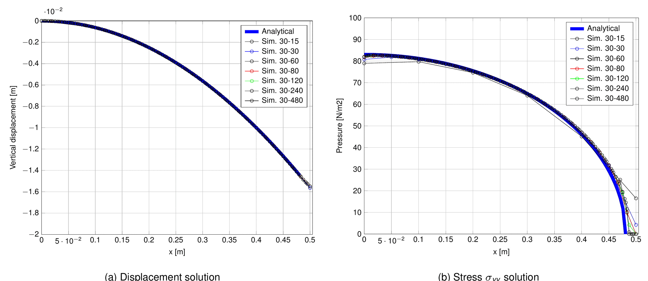
Figure: vertical displacement and contact pressure of the 2D Hertz benchmark for several mesh sizes compared with the analytical solution (thesis Fig. 4.50).
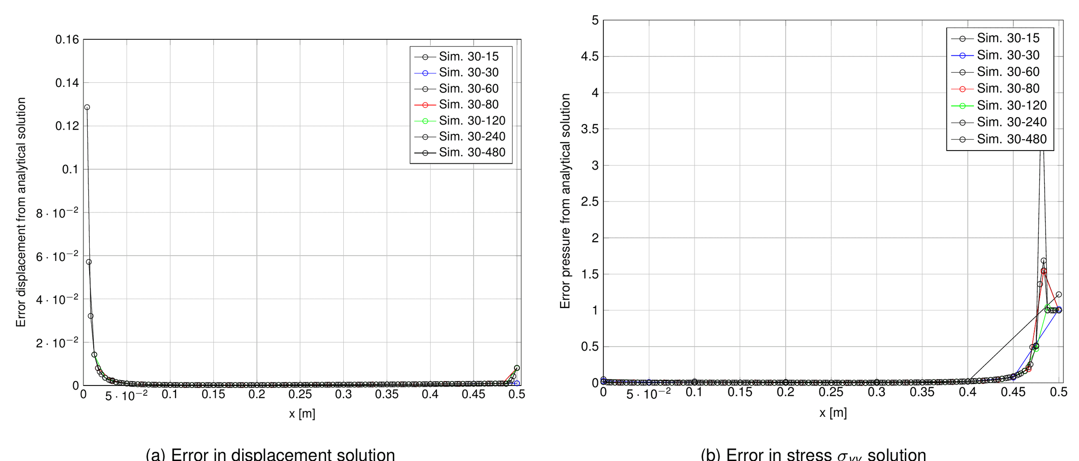
Figure: error with respect to the analytical solution for the same meshes (thesis Fig. 4.51).
A probe script equivalent to the one used here:
import math
import KratosMultiphysics as KM
import KratosMultiphysics.ContactStructuralMechanicsApplication as CSMA
# ... run the StructuralMechanicsAnalysis as in MainKratos.py, then:
mp = model["Structure"]
active = [n for n in mp.GetSubModelPart("Contact_Part").Nodes if n.Is(KM.SLAVE) and n.Is(KM.ACTIVE)]
p_max = max(-n.GetValue(CSMA.AUGMENTED_NORMAL_CONTACT_PRESSURE) for n in active)
a_num = 0.5 * (max(n.X for n in active) - min(n.X for n in active))
P = 0.2 * mp.ProcessInfo[KM.TIME] * 16.0                    # pressure x loaded width
E_star = 1.0 / ((1 - 0.3**2) / 2.0e2 + (1 - 0.3**2) / 2.0e12)
a = math.sqrt(4.0 * P * 8.0 / (math.pi * E_star)); p0 = 2.0 * P / (math.pi * a)
print(f"numerical: a ~ {a_num:.4f}, p_max = {p_max:.4f} | Hertz: a = {a:.4f}, p_max = {p0:.4f}")
Variations
All the following are test cases of the repository; the table lists the JSON changes with respect to the tutorial and the file to start from. They were all run while writing this page.
| Variant | Start from | Changes |
|---|---|---|
| Frictional contact (Coulomb) | tests/ALM_frictional_contact_test_2D/hyper_simple_patch_test_parameters.json (8-node patch test, 1 step) |
contact_settings.mortar_type: "ALMContactFrictional"; in the process "contact_type": "Frictional" and "friction_coefficients": {"0": 0.01}. The solver raises the buffer size to 3 and uses the vector multiplier VECTOR_LAGRANGE_MULTIPLIER; the convergence table gains stick/slip columns. Optional keys: tangent_factor, slip_threshold, contact_type: "FrictionalPureSlip". |
| 3D | tests/ALM_frictionless_contact_test_3D/3D_contact_simplest_patch_matching_test_parameters.json (16 nodes, 2 steps) |
domain_size: 3, 3D elements/conditions in the mesh; nothing changes in the contact blocks — the search picks the 3D3N, 3D4N or mixed conditions from the geometries. |
| Penalty | tests/penalty_frictionless_contact_test_2D/hyper_simple_patch_test_parameters.json |
mortar_type: "PenaltyContactFrictionless" and python_module: "penalty_contact_process" / process_name: "PenaltyContactProcess". No multiplier DoFs; the penetration is controlled by advance_ALM_parameters.stiffness_factor. |
| Components (vector multiplier) | the tutorial itself | mortar_type: "ALMContactFrictionlessComponents" and contact_type: "FrictionlessComponents"; the MixedULMLinearSolver condenses the multipliers (use_mixed_ulm_solver). Same results (23 active nodes, 4 and 3 iterations). |
| MPC contact | tests/mpc_contact_tests/2D_contact_simplest_patch_matching_test_parameters.json |
replace contact_settings by mpc_contact_settings: {"contact_type": "Frictionless"}, use convergence_criterion: "residual_criterion" and python_module: "mpc_contact_process" / process_name: "MPCContactProcess"; the interface is given as contact_model_part: {"0": ["Contact_Part_Slave", "Contact_Part_Master"]} with assume_master_slave: {"0": ["Contact_Part_Slave"]} (the name is historical: the listed part is the master). |
| Mesh tying | tests/mesh_tying_test/simple_patch_test_2D_parameters.json (24 nodes) |
mortar_type: "ComponentsMeshTying", python_module: "mesh_tying_process" / process_name: "MeshTyingProcess", interfaces in mesh_tying_model_part. |
| Axisymmetric | any 2D case | "alternative_formulations": {"axisymmetric": true} in the ALM/penalty process (uses …Axisym… conditions, THICKNESS in the properties). |
| Adaptive time stepping | any | contact_settings.adaptative_strategy: true with split_factor, max_number_splits — the step is subdivided when Newton fails. |
The complete Hertz benchmark of the thesis (finer meshes, cylinder–cylinder, frictional, 3D) is available in the Examples repository: validation/hertz and validation/hertz_full; see also Benchmarks.
Thesis figures © Vicente Mataix Ferrándiz, PhD thesis “Innovative mathematical and numerical models for studying the deformation of shells during industrial forming processes with the Finite Element Method”, UPC 2020, reproduced by the author. Figures marked “inspired by” are the author’s redrawings of the cited sources.