Sources. Thesis §4.4.1–4.4.3 (pp. 123–129: introduction, bounding volumes, OBB implementation, collision detection, SAT, tree structures), Figs. 4.26, 4.27, 4.29, 4.30, 4.32, 4.33; code:
custom_processes/base_contact_search_process.{h,cpp},custom_processes/simple_contact_search_process.cpp,custom_processes/advanced_contact_search_process.{h,cpp},custom_processes/contact_search_wrapper_process.cpp,custom_processes/find_intersected_geometrical_objects_with_obb_for_contact_search_process.{h,cpp},custom_processes/normal_check_process.cpp,custom_processes/master_slave_process.cpp,custom_utilities/interface_preprocess.{h,cpp},custom_utilities/contact_utilities.cpp,python_scripts/search_base_process.py,python_scripts/alm_contact_process.py,python_scripts/explicit_penalty_contact_process.py, Kratos corekratos/geometries/oriented_bounding_box.{h,cpp},kratos/spatial_containers/{kd_tree,bucket,tree,point_object}.h; teststests/cpp_tests/processes/test_search_process.cpp,tests/test_dynamic_search.py,tests/test_check_normals_process.py.
This page describes how the application decides which slave and master conditions may come into contact before the mortar conditions described in Frictionless contact and Conditions are ever assembled. The output of the search is the set of paired conditions stored in the ComputingContact sub-model-part; the gap checks and the activation of nodes are detailed in Gap computation and the automatic master/slave assignment in Self-contact.
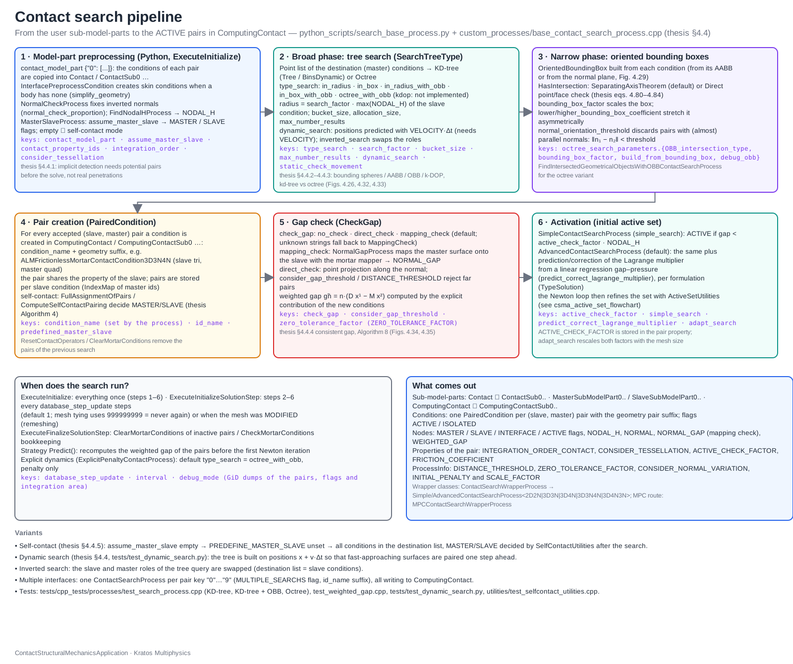
Figure: The contact search pipeline of the ContactStructuralMechanicsApplication, from the user model parts to the paired mortar conditions.
Explicit versus implicit detection (thesis §4.4.1)
The detection phase depends strongly on the time integration scheme:
- Explicit approach. The time step is very small, so it is enough to detect the bodies that have actually penetrated each other and apply repulsive forces. The focus is on real penetration, not on estimation.
- Implicit approach. The solution of the step depends on values that are not known yet, so potential pairings must be estimated in advance. Each potential pair introduces additional degrees of freedom (the Lagrange multipliers) and contributes to the left- and right-hand sides of the system.
The application targets the implicit approach, which makes the detection phase critical: superfluous pairs are not only expensive to assemble, they also degrade the conditioning of the system and the convergence of the active-set strategy. For \(n\) slave and \(m\) master conditions the naive brute-force search (test every master against every slave) costs \(\mathcal{O}(nm)\), which is unacceptable for meshes with a large number of contact faces. The goal of the search is therefore to find all proximate slave–master pairs with a cost close to \(\mathcal{O}(n \log m)\), which is what bounding volumes and tree structures provide.
The search pipeline of the application
Stage 0 – model parts and flags (SearchBaseProcess, Python)
All contact processes (ALMContactProcess, PenaltyContactProcess, ExplicitPenaltyContactProcess, MPCContactProcess, MeshTyingProcess) inherit from SearchBaseProcess in python_scripts/search_base_process.py. Its ExecuteInitialize builds the following hierarchy inside the structural model part (default name Structure):
| Sub-model-part | Created by | Content |
|---|---|---|
Contact |
SearchBaseProcess.ExecuteInitialize |
Union of all interface nodes and conditions; recreated from scratch when the root model part is flagged MODIFIED (remeshing) |
Contact/ContactSub<N> |
__generate_search_model_part_from_input_list (one per non-empty key "N" of contact_model_part), or __detect_skin when no model part is given |
Nodes and conditions of pair N |
Contact/ContactSub<N>/MasterSubModelPart<N> and SlaveSubModelPart<N> |
BaseContactSearchProcess::SetOriginDestinationModelParts (C++) |
Nodes/conditions flagged MASTER / SLAVE, consumed by NormalGapProcess and by the octree search |
ComputingContact and ComputingContact/ComputingContactSub<N> |
BaseContactSearchProcess constructor |
The paired mortar conditions actually assembled |
For every listed user model part the process sets the INTERFACE flag on nodes (and on conditions when present), assigns MASTER to everything and then SLAVE to the model parts listed in assume_master_slave["N"] (_assign_master_flags, _assign_slave_flags). If assume_master_slave["N"] is empty, predefined_master_slave becomes false and the master/slave roles are decided automatically (see Self-contact).
Stage 1 – interface conditions (InterfacePreprocessCondition)
When the interface model parts contain only nodes (the recommended input is conditions, but nodes are accepted), InterfacePreprocessCondition::GenerateInterfacePart scans the element faces whose nodes are all INTERFACE and creates LineCondition2D2N/LineCondition2D3N or SurfaceCondition3D3N/3D4N/3D6N/3D8N/3D9N conditions on them ("simplify_geometry": true forces the linear variants). Each new condition inherits the SLAVE/MASTER flag from its nodes (AssignMasterSlaveCondition) and either copies the element properties or uses contact_property_id. The conditions are then transferred to ContactSub<N> with FastTransferBetweenModelPartsProcess.
Stage 2 – normal check (NormalCheckProcess)
Mortar contact needs outward normals on both sides. NormalCheckProcess (defaults {"length_proportion": 0.1, "check_threshold": 5.0e-7}, length_proportion is set from normal_check_proportion) computes the unit normals with NormalCalculationUtils, offsets the center of every solid element face by length_proportion times its length along the normal and tests whether the offset point falls inside the parent element (IsInside with check_threshold). If it does, the face normal points inwards: the element and its conditions are flagged MARKER and inverted with MortarUtilities::InvertNormalForFlag, and the normals are recomputed. A second pass repeats the check node-wise on the averaged nodal normals. Slender elements (beams, shells, membranes) are skipped with an informative message. The process runs only when IS_RESTARTED == 0.
Stage 3 – master/slave flags on an existing Contact model part (MasterSlaveProcess)
When the Contact sub-model-part already exists (restart, or a user-provided interface), MasterSlaveProcess assigns the condition flags from the nodal ones: a condition whose nodes are all INTERFACE is SLAVE if all its nodes are SLAVE, otherwise MASTER; interface nodes and conditions are added to Contact.
Stage 4 – the C++ search process family
SearchBaseProcess._create_main_search instantiates CSMA.ContactSearchProcess (the Python name of ContactSearchWrapperProcess) for each pair N. The wrapper reads DOMAIN_SIZE and the number of nodes of the first MASTER and SLAVE conditions and creates the matching template instance:
| Geometry | simple_search: true |
simple_search: false (default) |
|---|---|---|
| 2D lines | SimpleContactSearchProcess<2,2> |
AdvancedContactSearchProcess<2,2> |
| 3D triangles | SimpleContactSearchProcess<3,3> |
AdvancedContactSearchProcess<3,3> |
| 3D quadrilaterals | SimpleContactSearchProcess<3,4> |
AdvancedContactSearchProcess<3,4> |
| Slave triangles / master quadrilaterals | SimpleContactSearchProcess<3,3,4> |
AdvancedContactSearchProcess<3,3,4> |
| Slave quadrilaterals / master triangles | SimpleContactSearchProcess<3,4,3> |
AdvancedContactSearchProcess<3,4,3> |
Both derive from BaseContactSearchProcess<TDim, TNumNodes, TNumNodesMaster>, which owns the whole algorithm; the derived classes only override the activation methods (SetActiveNode, ComputeActiveInactiveNodes, CheckPairing). MPCContactSearchProcess reuses the same base but creates ContactMasterSlaveConstraint objects instead of conditions. The constructor of the base class:
- requires the
Contactsub-model-part, validates the parameters and sets the local flagsINVERTED_SEARCH,PREDEFINE_MASTER_SLAVE,PURE_SLIP,MULTIPLE_SEARCHS(truewhenid_nameis not empty) andCREATE_AUXILIAR_CONDITIONS(truewhencondition_nameis not empty); - creates or cleans
ComputingContact[/ComputingContactSub<id_name>]; - builds the reference condition name
<condition_name>Condition<TDim>D<TNumNodes>N<final_string>(for instanceALMFrictionlessMortarContactCondition3D3N) and fetches it as aPairedConditionprototype; - resets
NORMAL_GAPto zero whencheck_gapisMappingCheckand deactivates all conditions ofContactSub<N>; - detects the
TypeSolutionfrom the nodal variables:VectorLagrangeMultiplier(VECTOR_LAGRANGE_MULTIPLIER),NormalContactStress(LAGRANGE_MULTIPLIER_CONTACT_PRESSURE),FrictionlessPenaltyMethod/FrictionalPenaltyMethod(WEIGHTED_GAPwithout multipliers),ScalarLagrangeMultiplier(SCALAR_LAGRANGE_MULTIPLIER) orOtherFrictionless/OtherFrictional.
Stage 5 – life cycle and database_step_update
The base process splits the work in the standard Kratos hooks (Execute() simply calls the three in sequence):
| Hook | Work |
|---|---|
ExecuteInitialize |
CheckContactModelParts (clones conditions that were already MARKER, so that shared conditions of several pairs get their own INDEX_MAP), CreatePointListMortar (fills the kd-tree point list with the master conditions, unless the octree is used), InitializeMortarConditions (gives every condition of ContactSub<N> an INDEX_MAP) |
ExecuteInitializeSolutionStep |
ClearMortarConditions then UpdateMortarConditions – the actual search |
ExecuteFinalizeSolutionStep |
ClearMortarConditions |
On the Python side, SearchBaseProcess.ExecuteInitializeSolutionStep only calls the C++ search when _compute_search() is true, i.e. when the process interval is active and either STEP == 1 or the internal counter database_step has reached search_parameters["database_step_update"] (default 1, search every step). When the search is skipped, all nodes and conditions of the contact model part are set ACTIVE = false, so increasing database_step_update disables contact in the intermediate steps; it is meant for problems where the pairing is known to be stable (mesh tying, small sliding). Before and after the search the MARKER flag of the nodes is reset: MARKER is set on nodes activated during the current search so that SetInactiveNode does not deactivate them again within the same call.
Stage 6 – broad phase: point list and trees (UpdateMortarConditions)
UpdateMortarConditions first refreshes the point list (UpdatePointListMortar: in the dynamic case it also applies the predicted displacement, see below), recomputes the unit normals of ContactSub<N> and, when the master/slave roles are not predefined, runs the self-contact pre-pairing. Then it dispatches on SearchTreeType:
type_search (JSON) |
SearchTreeType |
Broad-phase query |
|---|---|---|
"InRadius" / "in_radius" (C++ default) |
KdtreeInRadius = 0 |
Tree::SearchInRadius around the slave center with radius search_factor times the slave circumradius (Radius(): largest center-to-node distance) |
"InBox" / "in_box" |
KdtreeInBox = 1 |
Tree::SearchInBox with the slave bounding box whose extreme points are pushed along their normals by search_factor times the slave length (ContactUtilities::ScaleNode) |
"InRadiusWithOBB" / "in_radius_with_obb" (Python default) |
KdtreeInRadiusWithOBB = 2 |
As InRadius, plus an OBB intersection test between slave and each candidate master |
"InBoxWithOBB" / "in_box_with_obb" |
KdtreeInBoxWithOBB = 3 |
As InBox, plus the OBB test |
"OctreeWithOBB" / "octree_with_obb" (explicit default) |
OctreeWithOBB = 4 |
Octree of the master conditions built by FindIntersectedGeometricalObjectsWithOBBContactSearchProcess, OBB test in the leaves |
"KDOP" / "kdop" |
Kdop = 5 |
Not implemented – the constructor raises KDOP contact search: Not yet implemented |
Any other string silently falls back to KdtreeInRadius. The kd-tree branch (SearchUsingKDTree) builds a Tree<KDTreePartition<Bucket<3, PointObject<Condition>>>> over mPointListDestination (the master conditions, or the slave ones for an inverted search) with the given bucket_size, allocates a result vector of allocation_size entries per slave condition and calls PerformKDTreeSearch. The octree branch (SearchUsingOcTree) creates MasterSubModelPart<N>/SlaveSubModelPart<N>, forwards octree_search_parameters (with bounding_box_factor multiplied by the maximum NODAL_H of the two sides) to FindIntersectedGeometricalObjectsWithOBBContactSearchProcess and calls IdentifyNearEntitiesAndCheckEntityForIntersection for each active slave condition; conditions found to intersect are flagged SELECTED. The octree is not compatible with inverted_search (KRATOS_ERROR).
Stage 7 – narrow phase: OBB / SAT
In the *WithOBB variants an OrientedBoundingBox<TDim> is built for the slave (slave_obb) and for every candidate master, with half-lengths enlarged by bounding_box_factor times the maximum NODAL_H of the contact model part, and the candidate is discarded unless slave_obb.HasIntersection(master_obb); the intersection algorithm is selected by OBB_intersection_type (see Collision detection below). The octree process performs the same test inside MarkIfIntersected, additionally flagging the intersecting masters.
Stage 8 – pair filtering and creation
Every surviving candidate goes through CheckGeometricalObject / CheckCondition, which return Fail, AlreadyInTheMap or OK:
- a condition never pairs with itself;
- pairs whose center normals differ by less than
normal_orientation_threshold(default0.1, plus \(10^{-16}\)) are rejected – two faces looking in the same direction cannot be in contact (the same criterion drives the self-contact algorithm, Fig. 4.36); - when the roles are not predefined, or the candidate is itself a slave, the reverse pairing is rejected if it already exists in the candidate’s
INDEX_MAP; - a master already present in the slave’s
INDEX_MAPis reported asAlreadyInTheMap.
With check_gap = MappingCheck the accepted master ids are only stored in the slave INDEX_MAP; the pairs are created later by CheckPairing → CreateAuxiliaryConditions after the mapped gap has been computed. With NoCheck/DirectCheck, AddPotentialPairing decides immediately (see Gap computation). In both cases AddPairing clones the prototype PairedCondition with the slave geometry, the properties of the pair (contact_property_ids or the slave properties) and the master geometry as paired geometry, adds it to ComputingContactSub<N>, stores the new id in the INDEX_MAP (SetNewEntityId), copies the slave NORMAL, sets ACTIVE and calls Initialize. Ids continue after the maximum condition id of the main model part (GetMaximumConditionsIds). ResetContactOperators (called from the convergence criteria) removes the paired conditions that ended the step ACTIVE = false, or everything after a remeshing (MODIFIED).
Stage 9 – activation: simple versus advanced
The last part of UpdateMortarConditions resets the weighted variables (WEIGHTED_GAP, WEIGHTED_SLIP, WEIGHTED_SCALAR_RESIDUAL or WEIGHTED_VECTOR_RESIDUAL according to the TypeSolution), integrates them explicitly with ContactUtilities::ComputeExplicitContributionConditions and sets the nodal ACTIVE flags:
SimpleContactSearchProcessuses the base criterionNORMAL_GAP < GapThreshold * NODAL_HwithGapThreshold = 2.0e-3and, if the node penetrates, initializes the Lagrange multiplier with the penalty guess \(\lambda = \varepsilon A_i g_n / k\) (nodalINITIAL_PENALTYor the global one,NODAL_AREA,SCALE_FACTOR), written toVECTOR_LAGRANGE_MULTIPLIER,SCALAR_LAGRANGE_MULTIPLIERorLAGRANGE_MULTIPLIER_CONTACT_PRESSURE.AdvancedContactSearchProcessfirst setsDISTANCE_THRESHOLDto the maximum of the meanNODAL_Hof the master and slave sides, then activates a slave node whenNORMAL_GAP < ACTIVE_CHECK_FACTOR * DISTANCE_THRESHOLD, or when it is already active and its area-normalized weighted gap is below the same length;static_check_movement/consider_gap_thresholdwiden the threshold toGapThreshold = 2.0e-4for nodes whose weighted gap is not decreasing. Withpredict_correct_lagrange_multipliera linear regression pressure–gap over the active nodes (ComputeLinearRegressionGapPressure) is used to predict (Predict*MortarLM) or correct (Correct*MortarLM) the multiplier of each node.
Frictional problems also receive their SLIP flag here: nodes with zero FRICTION_COEFFICIENT or pure_slip are set SLIP, the others start in stick. All the thresholds are described in Gap computation.
Bounding volumes (thesis §4.4.2)
A bounding volume is a simple geometric envelope of a condition that makes the proximity test cheap. The thesis follows the classification of Dinas (Fig. 4.26): the trade-off is between the cost of the test and the tightness of the bound.
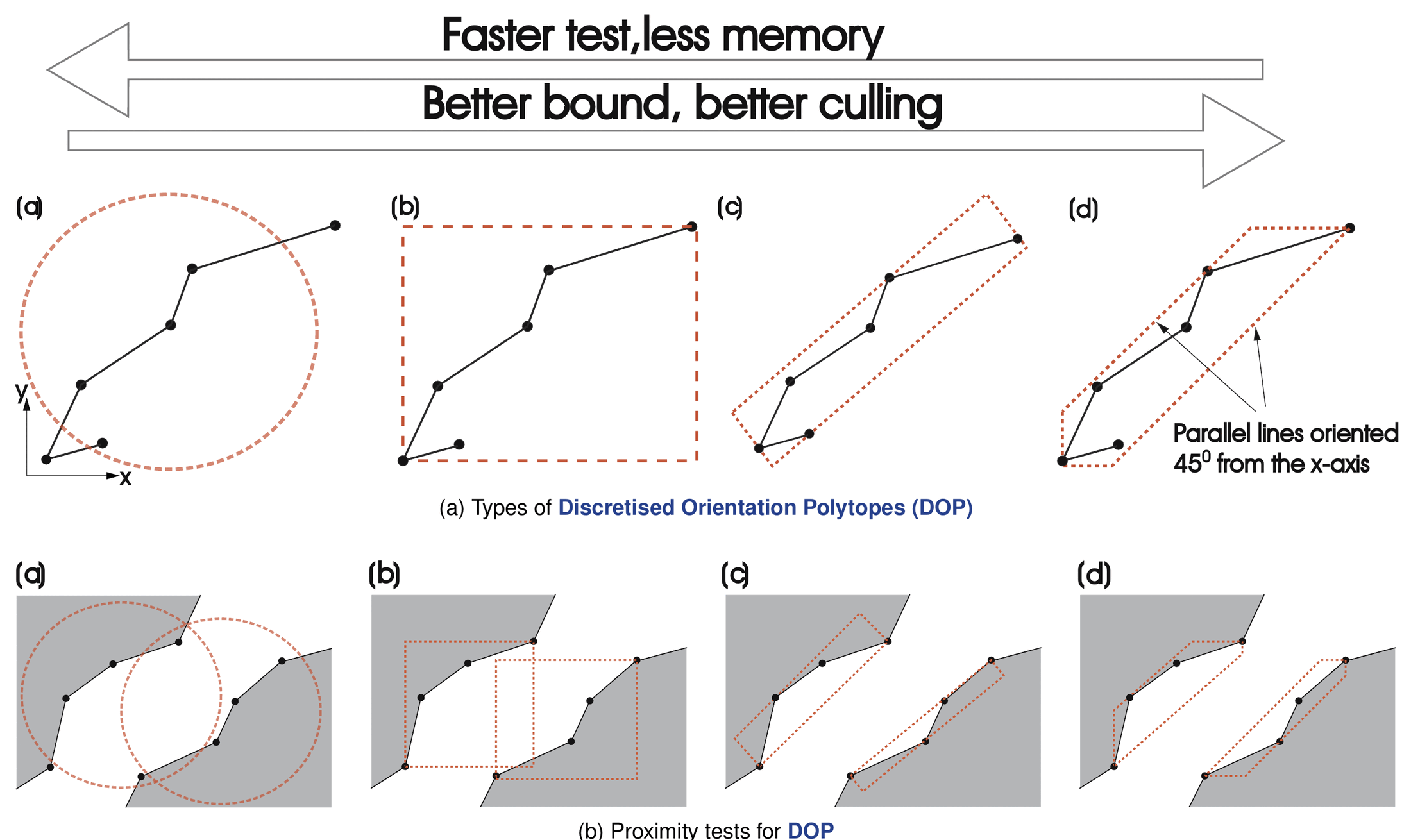
Figure: Types of bounding volumes and their proximity tests: (a) bounding sphere (radius search), (b) axis-aligned bounding box, (c) oriented bounding box, (d) discrete orientation polytope (thesis Fig. 4.26, inspired by Yang and Laursen 2008).
- Bounding sphere (BS) – the nodes inside a radius; the cheapest test and the loosest bound. This is what the plain
InRadiussearch does. - Axis-aligned bounding box (AABB) – a cuboid parallel to the Cartesian planes; still loose for inclined faces. This is the
InBoxsearch. - Oriented bounding box (OBB) – a box rotated with the face; much tighter, at the price of more computation and memory. This is the narrow phase of the
*WithOBBandOctreeWithOBBsearches. - k-DOP (discrete orientation polytope / convex hull) – always tighter than AABB and cheaper to update than OBB for deforming bodies, but not implemented (
SearchTreeType::Kdopis a placeholder).
The application originally used only the radius search; in order to capture all the pairs a large search_factor was needed, which produced many false potential pairs and impoverished the convergence of the active set (Fig. 4.27a). This is why the OBB was adopted as the intermediate solution and why the Python processes default to "in_radius_with_obb".
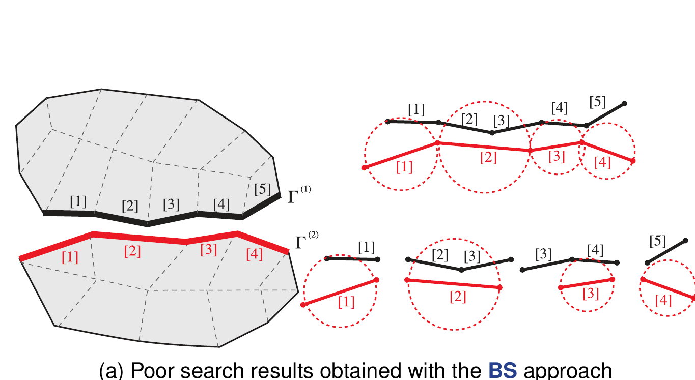
Figure: Poor search results obtained with the bounding-sphere approach: neighbouring faces are paired although they cannot come into contact (thesis Fig. 4.27a).
OBB definition and construction (thesis §4.4.2.1)
Following Eberly (GeometricTools), an OBB in \(\mathbb{R}^3\) is defined by a center \(\mathbf{C}\), a right-handed orthonormal set of axes \(\mathbf{A}_0, \mathbf{A}_1, \mathbf{A}_2\) and positive extents \(a_0, a_1, a_2\). The solid box is (thesis eq. 4.80a)
$$ \left\{ \mathbf{C} + \sum_{i=0}^{2} x_i \mathbf{A}_i \;:\; \vert x_i \vert \le \vert a_i \vert \ \text{ for all } i \right\} $$
and its eight vertices are (thesis eq. 4.80b)
$$ \mathbf{C} + \sum_{i=0}^{2} \sigma_i a_i \mathbf{A}_i, \qquad \vert \sigma_i \vert = 1 . $$
In the code the class is OrientedBoundingBox<TDim> (kratos/geometries/oriented_bounding_box.h) with members mPointCenter, mOrientationVectors and mHalfLength. The constructor OrientedBoundingBox(rGeometry, BoundingBoxFactor, BuildFromBoundingBox) offers the two construction strategies of the thesis for surface geometries:
- From the AABB (
build_from_bounding_box: true, default). \(\mathbf{A}_0\) is the normalized diagonal of the geometry bounding box and \(\mathbf{A}_1, \mathbf{A}_2\) complete an orthonormal basis (MathUtils::OrthonormalBasis). Simple, but for coplanar nodes the direction is arbitrary (Fig. 4.29a). - From the normal (
build_from_bounding_box: false). \(\mathbf{A}_0\) is the unit normal at the center; the nodes are rotated into the tangent plane (MortarUtilities::RotatePoint), the farthest node from the center defines \(\mathbf{A}_1\) and \(\mathbf{A}_2 = \mathbf{A}_1 \times \mathbf{A}_0\). The box is larger but oriented to the farthest point, which is less arbitrary (Fig. 4.29b). For solid geometries (WorkingSpaceDimension() == LocalSpaceDimension()) the first strategy is always used.
In both cases the extents are the maximum projections of the nodes on the axes plus BoundingBoxFactor, which is why bounding_box_factor is a relative quantity: the search process multiplies it by the maximum NODAL_H before building the boxes.
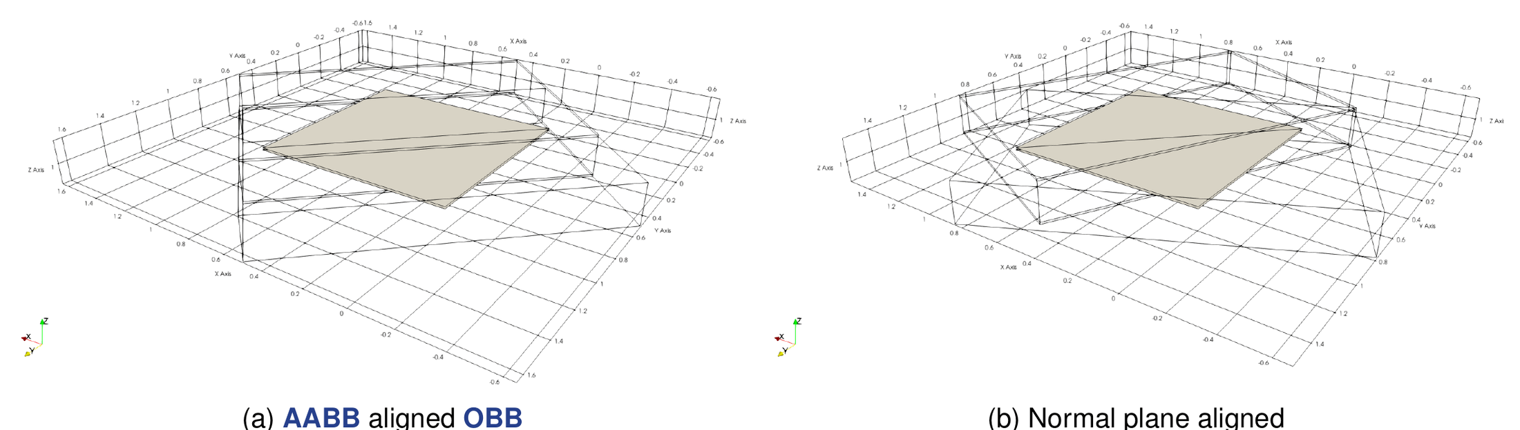
Figure: OBB from surfaces, build comparison: (a) AABB-aligned OBB, (b) normal-plane-aligned OBB (thesis Fig. 4.29).
Collision detection and the separating axis theorem (thesis §4.4.2.1)
Two algorithms are available for HasIntersection, selected by OBBHasIntersectionType ("Direct" or "SeparatingAxisTheorem" in OBB_intersection_type).
Direct check (DirectHasIntersection). First the vertices of one box are tested for inclusion in the other and vice versa (IsInside); the points are rotated to the axes of the target box (RotateNode2D/3D) so that the standard AABB inside test can be applied (CheckIsInside2D/3D). In 2D the vertex signs are (thesis eq. 4.81a)
$$ \text{sign}^{2D}_x = \begin{bmatrix} -1 & 1 & 1 & -1 \end{bmatrix}, \qquad \text{sign}^{2D}_y = \begin{bmatrix} -1 & -1 & 1 & 1 \end{bmatrix}, $$
each vertex \(i\) of the destination box is (thesis eq. 4.81b)
$$ \mathbf{x}^{aabb}_i = \mathbf{C}^{dest} + \text{sign}^{2D}_{xi} \, \mathbf{A}^{dest}_0 a^{dest}_0 + \text{sign}^{2D}_{yi} \, \mathbf{A}^{dest}_1 a^{dest}_1 , $$
and it lies inside the origin box when (thesis eq. 4.81c)
$$ \Vert \mathbf{x}^{aabb}_{xi} - C^{orig}_x \Vert \le a^{orig}_0 \quad \text{and} \quad \Vert \mathbf{x}^{aabb}_{yi} - C^{orig}_y \Vert \le a^{orig}_1 . $$
The 3D version uses the eight sign triplets of thesis eq. 4.82a, the vertex definition \(\mathbf{x}^{aabb}_i = \mathbf{C}^{dest} + \sum_k \text{sign}^{3D}_{ki} \mathbf{A}^{dest}_k a^{dest}_k\) (eq. 4.82b) and the three inequalities \(\Vert \mathbf{x}^{aabb}_{ki} - C^{orig}_k \Vert \le a^{orig}_k\) (eq. 4.82c). If no vertex is inside, the edges (2D, IntersectionUtilities::ComputeLineLineIntersection) or the faces (3D, Quadrilateral3D4::HasIntersection) of the equivalent geometries (GetEquivalentGeometry) are intersected pairwise. In total up to 24 checks are needed in 2D and 52 in 3D, although the loop stops at the first positive one.
Separating axis theorem (SeparatingAxisTheoremHasIntersection, default). Instead of testing nodes and faces, the SAT states that two convex sets are disjoint if and only if there is an axis \(\mathbf{n}\) on which their projections do not overlap (Figs. 4.30, 4.31). The candidate axes are the box axes and their pairwise cross products, in 2D (thesis eq. 4.83a)
$$ \mathbf{n} \in \left\{ \mathbf{A}^{dest}_0, \mathbf{A}^{dest}_1, \mathbf{A}^{orig}_0, \mathbf{A}^{orig}_1, \ \mathbf{A}^{dest}_0 \times \mathbf{A}^{orig}_0, \ \mathbf{A}^{dest}_0 \times \mathbf{A}^{orig}_1, \ \mathbf{A}^{dest}_1 \times \mathbf{A}^{orig}_0, \ \mathbf{A}^{dest}_1 \times \mathbf{A}^{orig}_1 \right\} $$
and in 3D the six axes plus the nine cross products \(\mathbf{A}^{dest}_i \times \mathbf{A}^{orig}_j\) (thesis eq. 4.83b). A plane with normal \(\mathbf{n}\) separates the boxes when the projected center distance exceeds the sum of the projected half-extents, in 2D (thesis eq. 4.84a)
$$ \Vert (\mathbf{C}^{dest} - \mathbf{C}^{orig}) \cdot \mathbf{n} \Vert \gt \Vert (\mathbf{A}^{dest}_0 a^{dest}_0) \cdot \mathbf{n} \Vert + \Vert (\mathbf{A}^{dest}_1 a^{dest}_1) \cdot \mathbf{n} \Vert + \Vert (\mathbf{A}^{orig}_0 a^{orig}_0) \cdot \mathbf{n} \Vert + \Vert (\mathbf{A}^{orig}_1 a^{orig}_1) \cdot \mathbf{n} \Vert $$
and in 3D with the third axis of each box added on the right-hand side (thesis eq. 4.84b). This is implemented in GetSeparatingPlane2D/3D; the number of checks drops to 8 in 2D and 15 in 3D, which is why the SAT is the default.
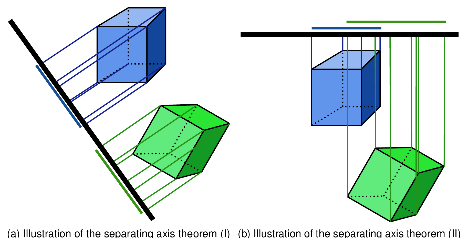
Figure: Illustration of the separating axis theorem: two boxes are disjoint if their projections on some axis do not overlap (thesis Fig. 4.30).
The octree_search_parameters block configures the OBB stage for every type_search (not only the octree, despite its name):
| Key | Default | Effect |
|---|---|---|
bounding_box_factor |
0.1 |
Relative enlargement of the OBB half-lengths (multiplied by the maximum NODAL_H); also enlarges the octree bounding box |
debug_obb |
false |
Writes the OBBs as auxiliary geometries (*_AUXILIAR_DEBUG_OBB sub-model-parts, debug builds) |
OBB_intersection_type |
"SeparatingAxisTheorem" |
"Direct" or "SeparatingAxisTheorem" |
build_from_bounding_box |
true |
OBB built from the AABB diagonal (true) or from the surface normal (false) |
lower_bounding_box_coefficient |
0.0 |
Octree only: extra extension of the lower corner of the global octree box in the thin directions (SetOctreeBoundingBox) |
higher_bounding_box_coefficient |
1.0 |
Octree only: same for the upper corner. Asymmetric values are useful when a flat interface lies on a coordinate plane |
Tree structures (thesis §4.4.3)
Bounding volumes make each pairwise test cheap; tree structures make the number of tests small. Fig. 4.32 compares the classical space-subdivision approaches: the uniform grid, the quadtree/octree, the kd-tree and the binary space partitioning tree.
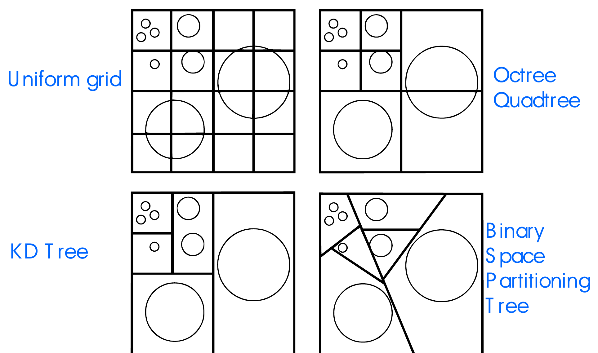
Figure: Space subdivision approaches: uniform grid, octree/quadtree, kd-tree, binary space partitioning tree (thesis Fig. 4.32).
A tree is a hierarchy of binary nodes (Fig. 4.33a): the top node is the root, nodes with children are parents, and the bottom ones are the leaves. The kd-tree recursively subdivides the space into disjoint hyper-rectangular cells; each tree node is associated with a box and the data points inside it, the root with the bounding box of all points (Fig. 4.33b). Besides the points, a kd-tree is defined by the bucket size (maximum number of points per leaf) and the splitting rule. The octree is the 3D analogue of the quadtree (each cell has eight children).
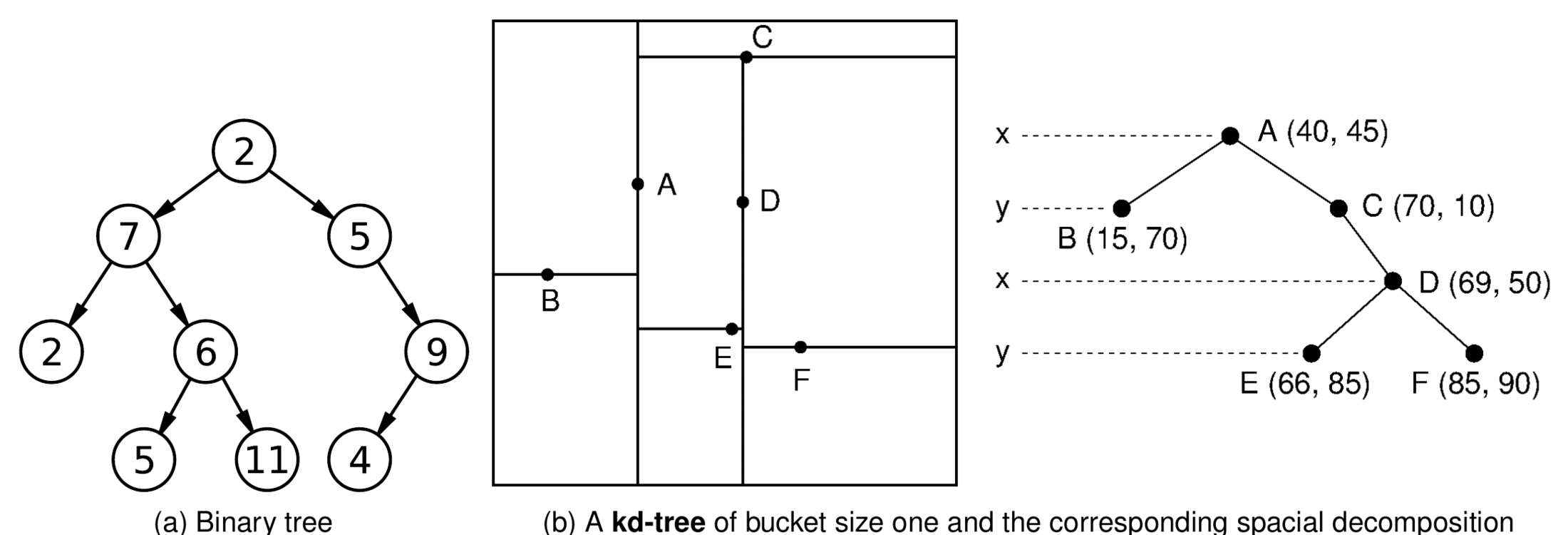
Figure: Tree structures: (a) binary tree, (b) a kd-tree of bucket size one and the corresponding spatial decomposition (thesis Fig. 4.33).
The application uses the trees already available in the Kratos core:
Tree<KDTreePartition<Bucket<3, PointObject<Condition>, PointVector>>>(kratos/spatial_containers/kd_tree.h,bucket.h,tree.h) for theKdtree*searches. The points arePointObject<Condition>(point_object.h), i.e. the centers of the master conditions, refreshed withUpdatePoint()at every search. The user controlsbucket_size(default4),allocation_size/max_number_results(default1000, size of the result buffer and upper bound on the number of candidates per slave) andsearch_factor(default3.5, multiplier of the radius or box).- The octree of
FindIntersectedGeometricalObjectsProcess(kratos/processes/find_intersected_geometrical_objects_process.h), specialized for contact inFindIntersectedGeometricalObjectsWithOBBContactSearchProcess, which overridesSetOctreeBoundingBox(the bounding box covers both the slave and the master model parts, enlarged bybounding_box_factorand the lower/higher coefficients) andMarkIfIntersected(onlySLAVEobjects are tested and both members of an intersecting pair are flaggedSELECTED).
Dynamic search and inverted search
Dynamic search (dynamic_search: true, effective only if VELOCITY is a nodal variable). The search is performed on the predicted configuration of the current step rather than on the converged configuration of the previous one. ContactUtilities::ComputeStepJump stores in DELTA_COORDINATES the displacement increment predicted from the velocities and the previous acceleration,
$$ \Delta \mathbf{x} = c_v \, \Delta t \, (\mathbf{v}^{n} + \mathbf{v}^{n-1}) + c_a \, \Delta t^2 \, \mathbf{a}^{n-1}, $$
with \(c_v = 0.5\), \(c_a = 0.5\) for a full jump and \(c_v = 0.25\), \(c_a = 0.125\) for the half jump used by GetHalfJumpCenter. The kd-tree query is centered at the half-jump center of the slave, and with MappingCheck the nodal coordinates are temporarily moved by DELTA_COORDINATES before the gap mapping and restored afterwards (UpdatePointListMortar, CheckPairing). static_check_movement complements this in the advanced activation by comparing WEIGHTED_GAP with its value in the previous step. tests/test_dynamic_search.py (test_dynamic_search_triangle, test_dynamic_search_quad) runs a falling block with ACCELERATION_X = -9.81 in the buffer, DELTA_TIME = 0.5 and ACTIVE_CHECK_FACTOR = 0.3, and compares the resulting NORMAL_GAP with reference JSON files.
Inverted search (inverted_search: true, or InvertSearch() at run time, flag INVERTED_SEARCH). All the Is(SLAVE) == !INVERTED_SEARCH tests of the base process flip, so the tree is built on the slave conditions and the master conditions are the query objects, and NormalGapProcess swaps the mapping direction (SearchOrientation = false). It is used to check the search from the master side; it is not available with the octree.
Multiple searches (id_name, flag MULTIPLE_SEARCHS). Each key N of contact_model_part produces an independent BaseContactSearchProcess operating on ContactSub<N> and ComputingContactSub<N>, which is how multi-body and multi-layer problems (ALMMultiLayerContactTest) are handled.
Explicit-dynamics defaults
ExplicitPenaltyContactProcess (used with contact_structural_mechanics_explicit_dynamic_solver.py) keeps the same search_parameters block but changes the default type_search to "octree_with_obb". In explicit analyses the time step is tiny and the search is called very often, so a search that does not require a global point list, works on actual penetration and shares the bounding box of both bodies is preferred; _compute_search still obeys database_step_update. Note that the octree path relies on MasterSubModelPart<N>/SlaveSubModelPart<N> and therefore requires predefined master/slave roles.
search_parameters reference
The block lives inside the contact process settings (alm_contact_process.py, penalty_contact_process.py, explicit_penalty_contact_process.py, mpc_contact_process.py, mesh_tying_process.py). Defaults are those of ALMContactProcess:
"search_parameters" : {
    "type_search"                         : "in_radius_with_obb",
    "simple_search"                       : false,
    "adapt_search"                        : false,
    "search_factor"                       : 3.5,
    "active_check_factor"                 : 0.01,
    "max_number_results"                  : 1000,
    "bucket_size"                         : 4,
    "dynamic_search"                      : false,
    "static_check_movement"               : false,
    "database_step_update"                : 1,
    "normal_orientation_threshold"        : 1.0e-1,
    "consider_gap_threshold"              : false,
    "debug_mode"                          : false,
    "predict_correct_lagrange_multiplier" : false,
    "check_gap"                           : "check_mapping",
    "octree_search_parameters" : {
        "bounding_box_factor"             : 0.1,
        "debug_obb"                       : false,
        "OBB_intersection_type"           : "SeparatingAxisTheorem",
        "build_from_bounding_box"         : true,
        "lower_bounding_box_coefficient"  : 0.0,
        "higher_bounding_box_coefficient" : 1.0
    }
}
| Key | Default | Meaning | Consuming code |
|---|---|---|---|
type_search |
"in_radius_with_obb" |
Broad/narrow phase combination, see the table of Stage 6 | BaseContactSearchProcess::ConvertSearchTree, CreatePointListMortar, UpdateMortarConditions |
simple_search |
false |
Select SimpleContactSearchProcess instead of AdvancedContactSearchProcess |
ContactSearchWrapperProcess (key removed before forwarding) |
adapt_search |
false |
Multiply search_factor and active_check_factor by the mesh size ratio \(h_{max}/h_{min}\) (ContactUtilities::CalculateRelativeSizeMesh) for strongly graded meshes |
SearchBaseProcess.ExecuteInitialize |
search_factor |
3.5 |
Radius (times the slave circumradius) or box extension (times the slave length) of the kd-tree query | PerformKDTreeSearch |
active_check_factor |
0.01 |
Written to ProcessInfo[ACTIVE_CHECK_FACTOR] and to the contact properties; fraction of DISTANCE_THRESHOLD (advanced) or of NODAL_H (direct check) below which a node is activated |
AdvancedContactSearchProcess::ComputeActiveInactiveNodes, AddPotentialPairing |
max_number_results |
1000 |
Forwarded as allocation_size: size of the kd-tree result buffer per slave |
SearchUsingKDTree, ClearDestinationListAndAssignFlags |
bucket_size |
4 |
kd-tree bucket size | SearchUsingKDTree |
dynamic_search |
false |
Search on the velocity-predicted configuration | UpdatePointListMortar, PerformKDTreeSearch, CheckPairing |
static_check_movement |
false |
Advanced activation: compare the weighted gap with the previous step | AdvancedContactSearchProcess::ComputeActiveInactiveNodes |
database_step_update |
1 |
Number of steps between two searches | SearchBaseProcess._compute_search, ExecuteFinalizeSolutionStep |
normal_orientation_threshold |
0.1 |
Minimum norm of the difference of the two center normals for a pair to be admissible | CheckGeometricalObject |
consider_gap_threshold |
false |
Advanced activation: enlarge the activation length to GapThreshold (2.0e-4) for nodes whose gap is not closing |
AdvancedContactSearchProcess::ComputeActiveInactiveNodes |
debug_mode |
false |
GiD dumps of flags (_debug_output), text files *_normal_debug_*.out, gap_active_nodes_debug_*.out, SELFCONTACT_* and the integrated area |
SearchBaseProcess, CreateDebugFile, ClearDestinationListAndAssignFlags |
predict_correct_lagrange_multiplier |
false |
Linear-regression prediction/correction of the multipliers of newly active nodes | AdvancedContactSearchProcess::ComputeActiveInactiveNodes, SetActiveNodeWithRegression |
check_gap |
"check_mapping" |
"NoCheck"/"no_check", "DirectCheck"/"direct_check", "MappingCheck"/"mapping_check"; unknown strings (including the Python default) resolve to MappingCheck |
BaseContactSearchProcess::ConvertCheckGap |
octree_search_parameters |
see above | OBB and octree configuration | SearchUsingKDTree, SearchUsingOcTree, FindIntersectedGeometricalObjectsWithOBBContactSearchProcess |
Keys that exist only at the C++ level (ContactSearchWrapperProcess::GetDefaultParameters) and are filled by SearchBaseProcess._create_search_parameters: condition_name and final_string (built from contact_type, normal_variation and the axisymmetric option, see Conditions), predefined_master_slave (from assume_master_slave), id_name (the pair key), allocation_size (from max_number_results), pure_slip (ALMContactProcess._set_additional_parameters) and inverted_search (C++ default false).
Note: _create_search_parameters forwards only simple_search, type_search, check_gap, bucket_size, search_factor, dynamic_search, static_check_movement, consider_gap_threshold, normal_orientation_threshold and debug_mode (plus allocation_size). The values of predict_correct_lagrange_multiplier and octree_search_parameters written in the Python search_parameters block are therefore not transmitted to the C++ process, which uses its own defaults (false, and the bounding_box_factor = 0.1 block). To change them from Python, create CSMA.ContactSearchProcess directly, as the C++ and Python tests do.
Tests
| Test | File | What it checks |
|---|---|---|
SearchProcessKDTree |
tests/cpp_tests/processes/test_search_process.cpp |
2D plane–cylinder problem (CreatePlaneCilynderProblemForSearch), "type_search": "InRadius", "check_gap": "MappingCheck", simple_search: true; asserts the exact content of the INDEX_MAP of each slave condition (2–3 masters for the central slaves, none for the extremes) |
SearchProcessKDTreeWithOBB |
same | Same problem with "InRadiusWithOBB" and bounding_box_factor = 0.1 |
SearchProcessOctree |
same | Same problem with "OctreeWithOBB" and "SeparatingAxisTheorem" |
test_dynamic_search_triangle / _quad |
tests/test_dynamic_search.py |
dynamic_search: true on a falling block; NORMAL_GAP compared with *_dynamic_search.json |
test_check_normals, test_check_normals_quads, test_check_normals_s_shape |
tests/test_check_normals_process.py |
NormalCheckProcess re-orients inverted normals on tetrahedra, hexahedra and the S-shape self-contact mesh |
InterfacePreprocessCondition2D, InterfacePreprocessCondition3D |
tests/cpp_tests/utilities/test_interface_preprocess_utilities.cpp |
Condition generation from INTERFACE nodes |
ALMMultiLayerContactTest, ComponentsALMMultiLayerContactTest |
tests/ValidationTests.py |
Several contact_model_part keys, i.e. multiple independent searches |
See also the test suite reference.
Notes and limitations
- The search loops over the slave conditions are serial (
// TODO: Make me parallel!!!); the kd-tree construction and the point updates are parallel. KDOPis declared inSearchTreeTypebut raises an error; use one of the OBB variants instead.- The octree search needs predefined master/slave roles and does not support
inverted_search. database_step_update > 1deactivates every contact node and condition in the steps without search; it is safe only when the contact state does not change between searches.- The Python default
"check_gap": "check_mapping"is not one of the strings recognized byConvertCheckGap; it works because the fallback isMappingCheck.
Thesis figures © Vicente Mataix Ferrándiz, PhD thesis “Innovative mathematical and numerical models for studying the deformation of shells during industrial forming processes with the Finite Element Method”, UPC 2020, reproduced by the author. Figures marked “inspired by” are the author’s redrawings of the cited sources.