Sources. Thesis Appendix A.3 “Mesh tying” (pp. 289–292) and the theory note shipped with the application,
automatic_differentiation/mesh_tying_mortar_condition/mesh_tying_mortar_condition.tex; code:custom_conditions/mesh_tying_mortar_condition.h/.cpp,python_scripts/mesh_tying_process.py,custom_strategies/custom_convergencecriterias/mesh_tying_mortar_criteria.h,custom_conditions/mpc_mortar_contact_condition.cpp(MPC tying variant).
Why mesh tying comes first
Mesh tying (also called tied contact or mortar domain decomposition) glues two independently meshed bodies along a common interface so that the displacement field is continuous across it, even if the nodes do not coincide. In the thesis it is presented as the base formulation of the contact method: it uses exactly the same ingredients (mortar projection, dual Lagrange multipliers, the operators \(\mathbf{D}\) and \(\mathbf{M}\)) but replaces the inequality (Karush–Kuhn–Tucker) constraints of unilateral contact by a plain equality constraint. The problem is therefore a standard saddle point problem with a known active set: every interface node is always “active”, there is no search for contact states, no penalty and no augmentation. This makes it the simplest way to understand and verify how the mortar integration works, which is the reason the application ships the mesh-tying condition next to the contact ones and tests it with the same patch tests.
Typical uses inside Kratos:
- connecting non-matching meshes of the same body (e.g. a fine region embedded in a coarse one, hexahedra tied to tetrahedra, triangles tied to quadrilaterals);
- tying dissimilar element types along an interface;
- “welded” interfaces between parts in an assembly, including a tension check variant that releases the tie when it works in traction (the MPC route, see below);
- tying of scalar fields (
TYING_VARIABLEdifferent fromDISPLACEMENT), since the condition is generic in the tied variable.
Strong formulation
On each subdomain \(\Omega_0^{(i)}\), \(i = 1, 2\), the initial boundary value problem of finite-deformation elastodynamics has to be satisfied (thesis eq. A.2, identical to the contact case, see Frictionless contact):
$$ \begin{aligned} & \mathrm{Div}\,\mathbf{P}^{(i)} + \hat{\mathbf{b}}_0^{(i)} = \rho_0^{(i)} \ddot{\mathbf{u}}^{(i)} && \text{in } \Omega_0^{(i)} \times [0, T] \\ & \mathbf{u}^{(i)} = \hat{\mathbf{u}}^{(i)} && \text{on } \Gamma_u^{(i)} \times [0, T] \\ & \mathbf{P}^{(i)} \cdot \mathbf{N}^{(i)} = \hat{\mathbf{t}}_0^{(i)} && \text{on } \Gamma_\sigma^{(i)} \times [0, T] \\ & \mathbf{u}^{(i)}(\mathbf{X}^{(i)}, 0) = \hat{\mathbf{u}}_0^{(i)}(\mathbf{X}^{(i)}), \quad \dot{\mathbf{u}}^{(i)}(\mathbf{X}^{(i)}, 0) = \hat{\dot{\mathbf{u}}}_0^{(i)}(\mathbf{X}^{(i)}) && \text{in } \Omega_0^{(i)} \end{aligned} $$
The only interface condition is the tied contact constraint, formulated in the reference configuration (thesis eq. A.2f):
$$ \mathbf{u}^{(1)} = \mathbf{u}^{(2)} \quad \text{on } \Gamma_c^{(i)} \times [0, T] $$
Compared with unilateral contact there is no gap function, no sign condition on the traction and no complementarity: the constraint is an equality that holds at all times on the whole interface. The balance of linear momentum across the interface is exploited by introducing a Lagrange multiplier vector field \(\boldsymbol{\lambda}\), which sets the basis for the mixed (saddle point) variational approach below.
Weak formulation
Solution and weighting spaces are the usual ones (thesis eq. A.3):
$$ \mathcal{U}^{(i)} = \left\{ \mathbf{u}^{(i)} \in H^1(\Omega) \,\middle|\, \mathbf{u}^{(i)} = \hat{\mathbf{u}}^{(i)} \text{ on } \Gamma_u^{(i)} \right\}, \qquad \mathcal{V}^{(i)} = \left\{ \delta\mathbf{u}^{(i)} \in H^1(\Omega) \,\middle|\, \delta\mathbf{u}^{(i)} = \mathbf{0} \text{ on } \Gamma_u^{(i)} \right\} $$
The Lagrange multiplier \(\boldsymbol{\lambda} = -\mathbf{t}_c^{(1)}\) represents the negative slave-side interface traction and lives in the dual space \(\mathcal{M}\) of the trace space of \(\mathcal{V}^{(1)}\), i.e. \(\mathcal{M} = H^{-1/2}(\Gamma_c)\). Find \(\mathbf{u}^{(i)} \in \mathcal{U}^{(i)}\) and \(\boldsymbol{\lambda} \in \mathcal{M}\) such that (thesis eq. A.4)
$$ \begin{aligned} -\delta\mathcal{W}_{kin}(\mathbf{u}^{(i)}, \delta\mathbf{u}^{(i)}) - \delta\mathcal{W}_{int,ext}(\mathbf{u}^{(i)}, \delta\mathbf{u}^{(i)}) - \delta\mathcal{W}_{mt}(\boldsymbol{\lambda}, \delta\mathbf{u}^{(i)}) &= 0 \quad \forall\, \delta\mathbf{u}^{(i)} \in \mathcal{V} \\ -\delta\mathcal{W}_{\lambda}(\mathbf{u}^{(i)}, \delta\boldsymbol{\lambda}) &= 0 \quad \forall\, \delta\boldsymbol{\lambda} \in \mathcal{M} \end{aligned} $$
with the kinetic, internal/external, interface and constraint contributions abbreviated as (thesis eq. A.5)
$$ \begin{aligned} -\delta\mathcal{W}_{kin} &= \sum_{i=1}^{2} \int_{\Omega_0^{(i)}} \rho_0^{(i)} \ddot{\mathbf{u}}^{(i)} \cdot \delta\mathbf{u}^{(i)} \, \mathrm{d}V_0 \\ -\delta\mathcal{W}_{int,ext} &= \sum_{i=1}^{2} \left[ \int_{\Omega_0^{(i)}} \left( \mathbf{S}^{(i)} : \delta\mathbf{E}^{(i)} - \hat{\mathbf{b}} \cdot \delta\mathbf{u}^{(i)} \right) \mathrm{d}V_0 - \int_{\Gamma_\sigma^{(i)}} \hat{\mathbf{t}}_0^{(i)} \cdot \delta\mathbf{u}^{(i)} \, \mathrm{d}A_0 \right] \\ -\delta\mathcal{W}_{mt} &= \int_{\Gamma_c^{(1)}} \boldsymbol{\lambda} \cdot \left( \delta\mathbf{u}^{(1)} - \delta\mathbf{u}^{(2)} \right) \mathrm{d}A_0 \\ -\delta\mathcal{W}_{\lambda} &= \int_{\Gamma_c^{(1)}} \delta\boldsymbol{\lambda} \cdot \left( \mathbf{u}^{(1)} - \mathbf{u}^{(2)} \right) \mathrm{d}A_0 \end{aligned} $$
The term \(\delta\mathcal{W}_{mt}\) is the virtual work of the unknown interface tractions \(\boldsymbol{\lambda} = -\mathbf{t}_c^{(1)} = \mathbf{t}_c^{(2)}\) and \(\delta\mathcal{W}_{\lambda}\) is the weak, variationally consistent enforcement of the tie. Both equations are equalities: this is exactly where mesh tying departs from contact, whose second equation is a variational inequality that requires an active-set strategy (see Frictionless contact). The choice of the discrete multiplier space \(\mathcal{M}_h\) is decisive for stability and optimal a-priori error bounds; the application uses dual Lagrange multipliers for it.
Discretisation and mortar operators
The dual Lagrange multipliers \(\Phi_j\) and the mortar operators are exactly those of the contact formulation and are derived in Mortar integration and dual Lagrange multipliers (thesis §4.3.3.4.1–4.3.3.4.2). Only the results needed here are repeated. The discrete multiplier is interpolated with the dual shape functions on the slave side,
$$ \boldsymbol{\lambda}_h = \sum_{j=1}^{m^{(1)}} \Phi_j\left(\xi^{(1)}, \eta^{(1)}\right) \boldsymbol{\lambda}_j , $$
where the \(\Phi_j\) satisfy the element-wise biorthogonality condition with the standard slave shape functions \(N_k^{(1)}\) and are obtained as \(\Phi_j = a_{jk} N_k^{(1)}\) with \(\mathbf{A}_e = \mathbf{D}_e \mathbf{M}_e^{-1}\) (thesis eqs. 4.20–4.24). Introducing the interpolation in the interface terms and integrating exclusively on the slave side \(\Gamma_{c,h}^{(1)}\) gives the two mortar matrices
$$ \begin{aligned} \mathbf{D}[j,k] &= D_{jk}\,\mathbf{I}_{n_{dim}} = \int_{\Gamma_{c,h}^{(1)}} \Phi_j N_k^{(1)} \, \mathrm{d}A_0 \, \mathbf{I}_{n_{dim}} = \sum_{g=1}^{n_{gp}} w_g \, \phi_{gj} N_{gk}^{(1)} J_g^{(1)} \, \mathbf{I}_{n_{dim}}, \\ \mathbf{M}[j,l] &= M_{jl}\,\mathbf{I}_{n_{dim}} = \int_{\Gamma_{c,h}^{(1)}} \Phi_j \left( N_l^{(2)} \circ \chi_h \right) \mathrm{d}A_0 \, \mathbf{I}_{n_{dim}} = \sum_{g=1}^{n_{gp}} w_g \, \phi_{gj} N_{gl}^{(2)} J_g^{(1)} \, \mathbf{I}_{n_{dim}}, \end{aligned} $$
with \(\chi_h\) the discrete interface mapping (projection of the slave Gauss point onto the master facet). Thanks to the biorthogonality, \(\mathbf{D}\) is diagonal. Both discrete interface contributions can then be written with the mortar tying operator \(\mathbf{B}_{mt}\):
$$ -\delta\mathcal{W}_{mt,h} = \delta\mathbf{d}_{\mathcal{S}}^T \mathbf{D}^T \boldsymbol{\lambda} - \delta\mathbf{d}_{\mathcal{M}}^T \mathbf{M}^T \boldsymbol{\lambda} = \delta\mathbf{d}^T \underbrace{\begin{bmatrix} \mathbf{0} \\ -\mathbf{M}^T \\ \mathbf{D}^T \end{bmatrix}}_{\mathbf{B}_{mt}^T} \boldsymbol{\lambda} = \delta\mathbf{d}^T \mathbf{f}_{mt}(\boldsymbol{\lambda}), \qquad -\delta\mathcal{W}_{\lambda,h} = \delta\boldsymbol{\lambda}^T \left( \mathbf{D}\,\mathbf{d}_{\mathcal{S}} - \mathbf{M}\,\mathbf{d}_{\mathcal{M}} \right) = \delta\boldsymbol{\lambda}^T \mathbf{g}_{mt}(\mathbf{d}). $$
\(\mathbf{f}_{mt} = \mathbf{B}_{mt}\boldsymbol{\lambda}\) is the vector of discrete tying forces on the slave and master sides, and \(\mathbf{g}_{mt}(\mathbf{d}) = \mathbf{D}\mathbf{d}_{\mathcal{S}} - \mathbf{M}\mathbf{d}_{\mathcal{M}}\) is the discrete (weighted) tying constraint — the mesh-tying counterpart of the weighted gap of the contact formulation.
Matrix form of the problem
With \(\mathcal{N}\) the DoFs not involved in the interface, \(\mathcal{M}\) the master and \(\mathcal{S}\) the slave interface DoFs, one Newton step of the coupled problem reads (thesis eq. A.6, .tex eq. 24)
$$ \begin{bmatrix} \mathbf{K}_{\mathcal{N}\mathcal{N}} & \mathbf{K}_{\mathcal{N}\mathcal{M}} & \mathbf{K}_{\mathcal{N}\mathcal{S}} & \mathbf{0} \\ \mathbf{K}_{\mathcal{M}\mathcal{N}} & \mathbf{K}_{\mathcal{M}\mathcal{M}} & \mathbf{0} & -\mathbf{M}^T \\ \mathbf{K}_{\mathcal{S}\mathcal{N}} & \mathbf{0} & \mathbf{K}_{\mathcal{S}\mathcal{S}} & \mathbf{D}^T \\ \mathbf{0} & -\mathbf{M} & \mathbf{D} & \mathbf{0} \end{bmatrix} \begin{bmatrix} \Delta\mathbf{d}_{\mathcal{N}} \\ \Delta\mathbf{d}_{\mathcal{M}} \\ \Delta\mathbf{d}_{\mathcal{S}} \\ \Delta\boldsymbol{\lambda} \end{bmatrix} = - \begin{bmatrix} \mathbf{r}_{\mathcal{N}} \\ \mathbf{r}_{\mathcal{M}} \\ \mathbf{r}_{\mathcal{S}} \\ \mathbf{r}_{\lambda} \end{bmatrix}, \qquad \mathbf{r}_{\lambda} = \mathbf{D}\,\mathbf{d}_{\mathcal{S}} - \mathbf{M}\,\mathbf{d}_{\mathcal{M}} . $$
Three remarks that carry over to the implementation:
- the interface blocks are constant as long as the interface geometry is frozen (the operators are computed from the reference configuration); the condition can therefore integrate \(\mathbf{D}\) and \(\mathbf{M}\) once and reuse them, and no linearisation of the operators is required;
- because \(\mathbf{D}\) is diagonal the system can be statically condensed (Popp 2012, thesis §4.3.3.4.4), removing the multipliers and producing a pure displacement formulation when the tied variable is the displacement — the same idea used by the MixedULMLinearSolver for contact and, in a different form, by the MPC tying variant described below;
- the multipliers have the meaning of interface tractions integrated with the dual basis: their nodal values are directly the tying reactions.
Implementation: MeshTyingMortarCondition
MeshTyingMortarCondition<TDim, TNumNodes, TNumNodesMaster> derives from PairedCondition (see Conditions) and is registered as
| Registered name | Slave geometry | Master geometry |
|---|---|---|
MeshTyingMortarCondition2D2N |
Line2D2 |
Line2D2 |
MeshTyingMortarCondition3D3N |
Triangle3D3 |
Triangle3D3 |
MeshTyingMortarCondition3D4N |
Quadrilateral3D4 |
Quadrilateral3D4 |
MeshTyingMortarCondition3D3N4N |
Triangle3D3 |
Quadrilateral3D4 |
MeshTyingMortarCondition3D4N3N |
Quadrilateral3D4 |
Triangle3D3 |
The Python process only asks for the base name MeshTyingMortar; the search process appends the geometry suffix of each pair it creates.
Generic tied variable. The condition does not hard-code displacements. The property TYING_VARIABLE (a string, default "DISPLACEMENT") is resolved in Initialize(): a scalar variable is tied with a SCALAR_LAGRANGE_MULTIPLIER DoF per slave node, an array_1d variable with the VECTOR_LAGRANGE_MULTIPLIER_X/Y/Z DoFs. The resolved variable pointers are kept in the members mpDoFVariables (tied DoFs) and mpLMVariables (multiplier DoFs), and dof_size = mpDoFVariables.size() is the number of tied components per node.
Operators computed once. Initialize() performs the exact mortar segmentation (ExactMortarIntegrationUtility, with tessellation enabled by default for tying), computes the dual coefficient matrix \(\mathbf{A}_e\) with CalculateAe and integrates \(\mathbf{D}\) and \(\mathbf{M}\) into the member mMortarConditionMatrices. Nothing is recomputed during the Newton iterations, consistent with the constant interface blocks of the matrix form above. Because the operators are not linearised, no automatic differentiation is involved: the generator kept in automatic_differentiation/mesh_tying_mortar_condition/ is marked legacy and the condition’s local system is hand-written.
Local system. With the DoF ordering [ MASTER, SLAVE, LM ], CalculateLocalLHS fills only the off-diagonal coupling blocks and CalculateLocalRHS the corresponding residuals (lines 528–650 of the .cpp):
$$ \mathbf{K}_{loc} = k \begin{bmatrix} \mathbf{0} & \mathbf{0} & -\mathbf{M}^T \\ \mathbf{0} & \mathbf{0} & \mathbf{D}^T \\ -\mathbf{M} & \mathbf{D} & \mathbf{0} \end{bmatrix}, \qquad \mathbf{r}_{loc} = k \begin{bmatrix} \mathbf{M}^T \boldsymbol{\lambda} \\ -\mathbf{D}^T \boldsymbol{\lambda} \\ -\left( \mathbf{D}\,\mathbf{u}^{(1)} - \mathbf{M}\,\mathbf{u}^{(2)} \right) \end{bmatrix}, $$
where each scalar entry \(D_{jk}\), \(M_{jl}\) is expanded to dof_size components. The factor \(k\) is the SCALE_FACTOR of the ProcessInfo (falling back to BUILD_SCALE_FACTOR, then to 1); it only improves the conditioning of the saddle point system and does not change the solution. The Python process computes it automatically from the mean Young modulus and mesh size with ALMVariablesCalculationProcess (compute_penalty disabled) unless manual_scale_factor is set — the same calibration as the contact scale factor (thesis eq. 4.11).
Integration order. GetIntegrationMethod() maps the property INTEGRATION_ORDER_CONTACT (1–5) to the Gauss rules GI_GAUSS_1 … GI_GAUSS_5; the default is 2. Since the tied integrand is a product of two linear shape functions on each integration cell, low orders already integrate it exactly; the Taylor-patch study of thesis App. A.2.2.2 shows that the segmentation (exact integration cells) matters much more than the number of Gauss points.
Convergence criterion. MeshTyingMortarConvergenceCriteria (mesh_tying_mortar_criteria) has no active set to check: it only prints its column in the convergence table and always returns converged. The displacement/LM criteria of the contact factory (contact_displacement_criterion, contact_residual_criterion, …) are used unchanged; the solver’s mortar_type is ScalarMeshTying or ComponentsMeshTying, which adds the SCALAR_LAGRANGE_MULTIPLIER or VECTOR_LAGRANGE_MULTIPLIER variables and DoFs (with reactions WEIGHTED_SCALAR_RESIDUAL / WEIGHTED_VECTOR_RESIDUAL_X/Y/Z) in auxiliary_methods_solvers.py.
Note. In the application constructor the prototypes of
MeshTyingMortarCondition3D3N4Nand3D4N3Nare built with matching geometry pairs (triangle/triangle and quadrilateral/quadrilateral) instead of the mixed pairs used by the contact families; the created conditions still receive the true pair geometries from the search, so the mixed tying tests work, but the prototype geometries are not representative (see Conditions).
Usage: mesh_tying_process.py
MeshTyingProcess derives from SearchBaseProcess and reuses the whole search pipeline (see Search pipeline); the only differences are the condition name, the absence of any activation check and the large default database_step_update, which freezes the pairs after the first step. Defaults:
{
    "help"                         : "This class is used in order to compute the a mortar mesh tying formulation. This class constructs the model parts containing the mesh tying conditions and initializes parameters and variables related with the mesh tying. The class creates search utilities to be used to create the tying pairs",
    "model_part_name"              : "Structure",
    "mesh_tying_model_part"        : {"0":[],"1":[],"2":[],"3":[],"4":[],"5":[],"6":[],"7":[],"8":[],"9":[]},
    "assume_master_slave"          : {"0":[],"1":[],"2":[],"3":[],"4":[],"5":[],"6":[],"7":[],"8":[],"9":[]},
    "mesh_tying_property_ids"      : {"0": 0,"1": 0,"2": 0,"3": 0,"4": 0,"5": 0,"6": 0,"7": 0,"8": 0,"9": 0},
    "interval"                     : [0.0,"End"],
    "variable_name"                : "DISPLACEMENT",
    "consider_static_condensation" : false,
    "zero_tolerance_factor"        : 1.0,
    "integration_order"            : 2,
    "consider_tessellation"        : true,
    "normal_check_proportion"      : 0.1,
    "search_parameters"            : {
        "type_search"                 : "in_radius_with_obb",
        "search_factor"               : 3.5,
        "active_check_factor"         : 0.01,
        "max_number_results"          : 1000,
        "bucket_size"                 : 4,
        "dynamic_search"              : false,
        "database_step_update"        : 999999999,
        "debug_mode"                  : false,
        "check_gap"                   : "check_mapping",
        "octree_search_parameters"    : {
            "bounding_box_factor"             : 0.1,
            "debug_obb"                       : false,
            "OBB_intersection_type"           : "SeparatingAxisTheorem",
            "lower_bounding_box_coefficient"  : 0.0,
            "higher_bounding_box_coefficient" : 1.0
        }
    },
    "scale_factor_parameters"      : {
        "manual_scale_factor"         : false,
        "stiffness_factor"            : 1.0,
        "scale_factor"                : 1.0e0
    }
}
| Key | Meaning |
|---|---|
mesh_tying_model_part |
Up to ten interface pairs ("0" … "9"), each a list of the sub-model-parts whose conditions form one tied interface (the two sides of the interface). |
assume_master_slave |
For each pair, the sub-model-part(s) that play the master role; the rest of the pair is slave. Empty lists let MasterSlaveProcess decide. |
mesh_tying_property_ids |
Property id used for the created conditions of each pair (0 = a new property copied from the elements). |
variable_name |
Tied variable; a scalar variable selects ScalarMeshTying (one SCALAR_LAGRANGE_MULTIPLIER per slave node), an array_1d variable ComponentsMeshTying. Written into the property TYING_VARIABLE. |
consider_static_condensation |
Runs AssignParentElementConditionsProcess so that every tying condition knows its parent element (PARENT_ELEMENT), the information needed to condense the interface statically. |
integration_order, consider_tessellation |
Property values INTEGRATION_ORDER_CONTACT and CONSIDER_TESSELLATION read by the condition; tessellation is on by default for tying (it improves the exact segmentation on warped quadrilaterals). |
search_parameters |
Same meaning as for contact; database_step_update = 999999999 keeps the pairing fixed after the first step, which is what a tied interface needs. |
scale_factor_parameters |
Manual or automatic (ALMVariablesCalculationProcess, \(k \approx\) stiffness_factor \(\cdot E_{mean}/h_{mean}\)) scale factor \(k\) of the coupling blocks. |
The solver must expose the multiplier DoFs, which happens automatically when the process writes mortar_type into solver_settings.contact_settings; a minimal ProjectParameters.json fragment is
"solver_settings" : {
    "solver_type" : "Static",
    "contact_settings" : { "mortar_type" : "ComponentsMeshTying" },
    "convergence_criterion" : "contact_residual_criterion"
},
"processes" : {
    "contact_process_list" : [{
        "python_module" : "mesh_tying_process",
        "kratos_module" : "KratosMultiphysics.ContactStructuralMechanicsApplication",
        "process_name"  : "MeshTyingProcess",
        "Parameters"    : {
            "model_part_name"       : "Structure",
            "mesh_tying_model_part" : { "0" : ["Contact_Part_1", "Contact_Part_2"] },
            "assume_master_slave"   : { "0" : ["Parts_Parts_Auto2"] }
        }
    }]
}
The complete key-by-key reference is in Contact process settings.
The MPC tying variant (tying with tension check)
The multipoint-constraint route of the application (see Frictional laws and MPC constraint and thesis App. D.5) offers a second way to tie meshes without Lagrange-multiplier DoFs. When an MPCMortarContactCondition carries the RIGID flag, its InitializeNonLinearIteration calls UpdateConstraintTying, which builds the linear relation
$$ \mathbf{u}_{\mathcal{S}} = \mathbf{D}^{-1}\mathbf{M}\,\mathbf{u}_{\mathcal{M}} $$
between slave and master displacements (trivial inversion of the diagonal \(\mathbf{D}\) with dual multipliers) and writes it into the attached ContactMasterSlaveConstraint. The builder-and-solver then eliminates the slave DoFs (master–slave elimination, thesis eq. D.12), giving a pure displacement system. The “tension check” of the feature list refers to the MPCContactCriteria, which maps the master reactions onto the slave side and releases a tied node when the interface works in traction beyond reaction_check_stiffness_factor \(\cdot E\); a plain tie keeps all nodes constrained. This variant is driven by mpc_contact_process.py (contact_type and the RIGID flag on the conditions) rather than by mesh_tying_process.py.
Numerical example (thesis A.3.5)
The thesis validates the formulation with an L-shaped hyperelastic solid whose corner region is meshed as a separate body; the two meshes do not match along the circular interface. Both solids are Neo-Hookean in a Total Lagrangian frame with the properties of thesis Table A.1:
| Solid 1 | Solid 2 | |
|---|---|---|
| Young modulus \(E\) | \(2 \times 10^8\) Pa | \(2 \times 10^8\) Pa |
| Poisson ratio \(\nu\) | 0.35 | 0.35 |
A vertical displacement equal to \(t\) (in metres, \(t \in [0, 2]\) s) is imposed on the upper corner while the lower corner is fixed. The interface stays continuous throughout the large-displacement solution: from a practical point of view the two bodies behave as one continuous mesh, which is exactly the behaviour of the original mortar domain decomposition methods (Wohlmuth 2001, Toselli–Widlund 2005).
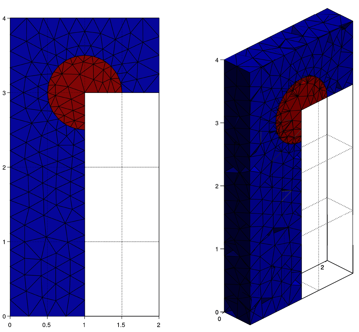
Figure: mesh of the L-shaped mesh-tying example, front and perspective views; the circular corner body is meshed independently (thesis Fig. A.7).
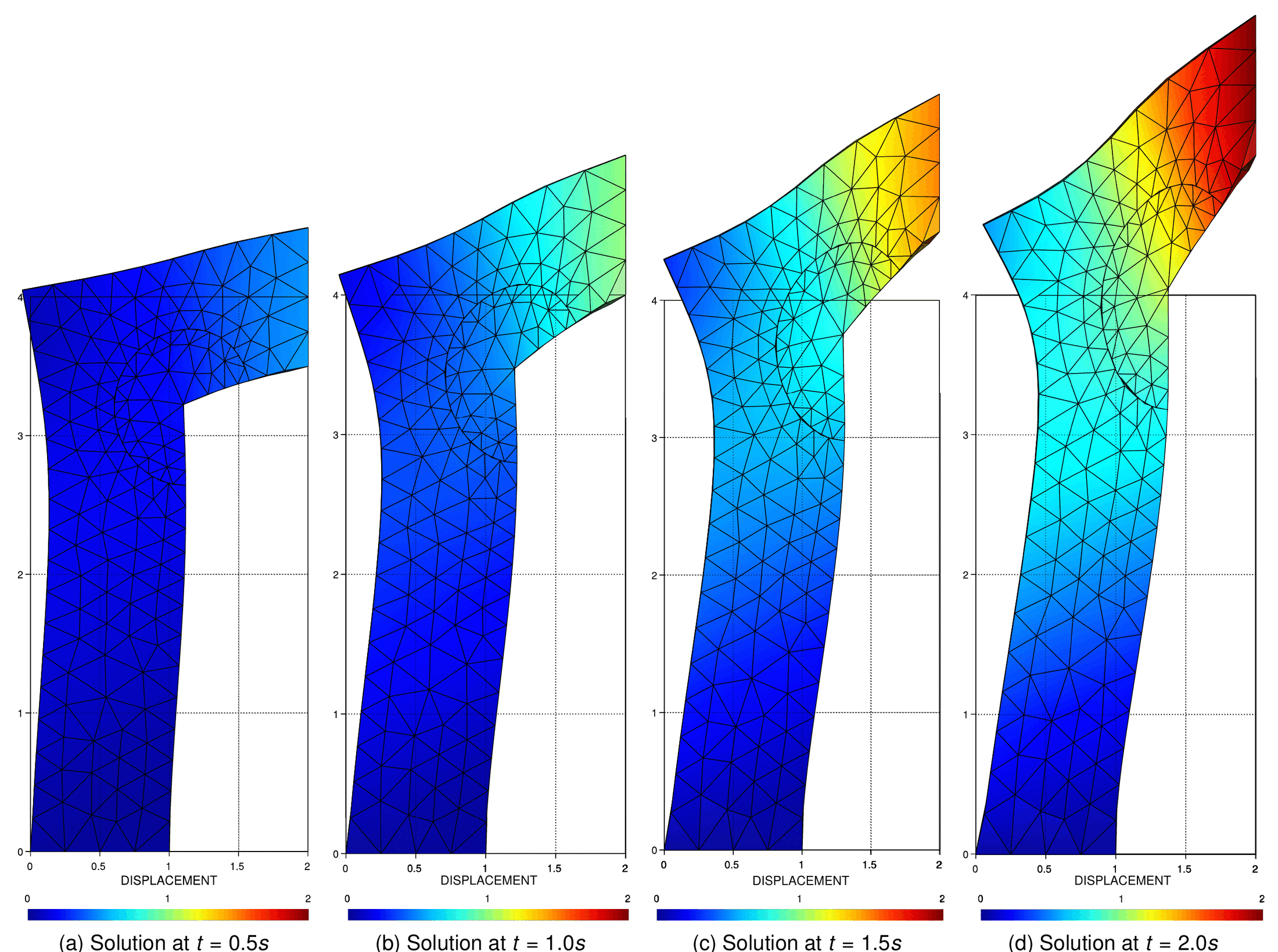
Figure: displacement solution at $$t = 0.5$$ s and $$t = 1.0$$ s; the non-matching interface remains continuous (thesis Fig. A.8).
The Taylor patch test used in App. A.2.2.2 to compare exact segmentation with collocation is also a tied problem; its figures are shown in Mortar integration and dual Lagrange multipliers.
Where it is tested
| Test class (suite) | Parameters file in tests/mesh_tying_test/ |
What it checks |
|---|---|---|
SimplePatchTestTwoDMeshTying (small) |
simple_patch_test_2D_parameters.json |
2D non-matching patch test, constant stress transmitted through the tie |
SimpleSlopePatchTestTwoDMeshTying (small) |
hyper_simple_slope_patch_test_2D_parameters.json |
2D sloped interface |
SimplestPatchTestThreeDMeshTying (small) |
3D_contact_simplest_patch_matching_test_parameters.json |
3D matching hexahedra/tetrahedra interface |
SimplestPatchTestThreeDTriQuadMeshTying, SimplestPatchTestThreeDQuadTriMeshTying (nightly) |
3D_contact_simplest_patch_matching_triquad_test_parameters.json, ..._quadtri_... |
mixed triangle/quadrilateral pairs (3D3N4N, 3D4N3N) |
SimplePatchTestThreeDMeshTying (nightly) |
simple_patch_test_3D_parameters.json |
3D non-matching patch test |
MeshTyingValidationTest (validation) |
mesh_tying_validation_test_parameters.json |
the L-shaped example of thesis A.3.5 |
LargeDisplacementPatchTestHexa (validation) |
3D_contact_patch_test_large_disp_hexa_parameters.json |
large-displacement tied hexahedra |
C++ MeshTyingCondition1, MeshTyingCondition2 |
tests/cpp_tests/conditions/test_mesh_tying_condition.cpp |
local LHS/RHS of the condition |
See Test suite reference for how to run them.
Further reading
- A. Popp, Mortar Methods for Computational Contact Mechanics and General Interface Problems, PhD thesis, TU München, 2012 — mesh tying with dual Lagrange multipliers and its static condensation.
- B. I. Wohlmuth, Discretization Methods and Iterative Solvers Based on Domain Decomposition, Springer, 2001 — the original mortar domain decomposition.
- M. A. Puso, A 3D mortar method for solid mechanics, IJNME 59 (2004) — mortar tying of non-matching 3D meshes.
- V. Mataix Ferrándiz, PhD thesis, UPC 2020 — Appendix A.3.
Thesis figures © Vicente Mataix Ferrándiz, PhD thesis “Innovative mathematical and numerical models for studying the deformation of shells during industrial forming processes with the Finite Element Method”, UPC 2020, reproduced by the author. Figures marked “inspired by” are the author’s redrawings of the cited sources.