Sources. Thesis §4.3.3.4.4 (pp. 110–111, eqs. 4.37–4.40); code:
custom_strategies/custom_builder_and_solvers/contact_residualbased_block_builder_and_solver.h,contact_residualbased_elimination_builder_and_solver.h,contact_residualbased_elimination_builder_and_solver_with_constraints.h,custom_linear_solvers/mixedulm_linear_solver.h,custom_python/add_custom_strategies_to_python.cpp,custom_python/add_custom_linear_solvers_to_python.cpp,python_scripts/auxiliary_methods_solvers.py(AuxiliaryCreateLinearSolver),python_scripts/contact_structural_mechanics_static_solver.py(_CreateBuilderAndSolver),tests/cpp_tests/linear_solvers/test_mixedulm_linear_solver.cpp.
A mortar contact problem with Lagrange multipliers produces a saddle-point system: the multiplier DoFs have a zero diagonal in the stiffness matrix, inactive slave nodes carry multipliers that must be forced to zero, and the set of active constraints changes from one iteration to the next. The application handles this at two levels. The builder-and-solvers (header-only classes in custom_strategies/custom_builder_and_solvers/) fix the DoF bookkeeping so that the assembled matrix is never singular for a trivial reason (isolated slave nodes, fixed slave displacements, multi-point constraints on interface nodes). The MixedULMLinearSolver (custom_linear_solvers/mixedulm_linear_solver.h) then exploits the diagonal structure that the dual Lagrange multipliers give to the multiplier block to condense it out and hand a displacement-only, better-conditioned matrix to a standard inner solver. Both are exposed to Python through the bindings in custom_python/ and selected automatically by the contact solvers described in the Solver settings reference. The convergence loop that calls them is described in Strategies and convergence criteria.
Builder and solvers
| Class | File | Name() |
Python name | Base class |
|---|---|---|---|---|
ContactResidualBasedBlockBuilderAndSolver |
contact_residualbased_block_builder_and_solver.h |
contact_block_builder_and_solver |
ContactResidualBasedBlockBuilderAndSolver |
ResidualBasedBlockBuilderAndSolver |
ContactResidualBasedEliminationBuilderAndSolver |
contact_residualbased_elimination_builder_and_solver.h |
contact_residual_elimination_builder_and_solver |
ContactResidualBasedEliminationBuilderAndSolver |
ResidualBasedEliminationBuilderAndSolver |
ContactResidualBasedEliminationBuilderAndSolverWithConstraints |
contact_residualbased_elimination_builder_and_solver_with_constraints.h |
contact_residual_elimination_builder_and_solver_with_constraints |
ContactResidualBasedEliminationBuilderAndSolverWithConstraints |
ResidualBasedEliminationBuilderAndSolverWithConstraints |
Each class only has {"name" : "<Name()>"} as its own default parameters, merged with the base defaults; all of them are templates on TSparseSpace, TDenseSpace, TLinearSolver and are instantiated for the Ublas spaces in add_custom_strategies_to_python.cpp. The Python constructors take the linear solver (CSMA.ContactResidualBasedBlockBuilderAndSolver(linear_solver)).
Block builder-and-solver: isolated nodes
Source. A block builder-and-solver keeps every DoF in the system, fixed ones included, and imposes Dirichlet conditions by zeroing rows and columns and writing the diagonal. With Lagrange multipliers this exposes a problem: a slave node whose pair conditions have an empty (or negligible) mortar integration domain contributes nothing to the rows of its multiplier DoFs, so the block matrix has zero rows and the linear solver fails. MortarContactCondition::CalculateConditionSystem flags such pair conditions ISOLATED and zeroes their local system (mortar_contact_condition.cpp:422); the builder-and-solver turns the condition flag into a nodal flag and fixes the affected multipliers for the duration of the Dirichlet treatment.
Both ApplyDirichletConditions and BuildRHS are overridden with the same pattern:
FixIsolatedNodes(rModelPart);
BaseType::ApplyDirichletConditions(...);   // or BaseType::BuildRHS(...)
FreeIsolatedNodes(rModelPart);
FixIsolatedNodes (lines 292-337) requires the Contact and ComputingContact sub-model-parts to exist (KRATOS_ERROR_IF_NOT), resets VISITED and ISOLATED on the Contact nodes, and loops over the pair conditions of ComputingContact: for every node of the parent (slave) geometry, the first visit copies the ISOLATED state of the condition, and subsequent visits AND it with the current nodal value (with SetLock / UnSetLock because the loop is parallel). A slave node is therefore ISOLATED only when all the pair conditions it belongs to are isolated, that is when it has no master in front of it at all. For those nodes the multiplier DoFs are fixed: LAGRANGE_MULTIPLIER_CONTACT_PRESSURE for the scalar formulation, or the three VECTOR_LAGRANGE_MULTIPLIER_X/Y/Z for the components and frictional ones. FreeIsolatedNodes (lines 343-361) releases the same DoFs afterwards, so that from the point of view of the strategy and of the convergence criteria the DoFs are still free, and a node that finds a master in the next search does not need to be re-declared. Since the fixed DoFs receive a unit diagonal and a zero right-hand side, the multiplier increment of an isolated node is zero and its multiplier keeps the value of the previous step (usually zero, since isolated nodes are inactive).
This is the default builder-and-solver of the contact solvers (builder_and_solver_settings.type is block by default in StructuralMechanicsApplication/python_scripts/structural_mechanics_solver.py), and the one that works together with the MixedULMLinearSolver in the standard configuration (rModelPart.IsNot(TO_SPLIT) branch of ProvideAdditionalData, see below). See also the description of the ISOLATED flag in the Architecture page.
Elimination builder-and-solver: consistent fixity of multipliers
Source. An elimination builder-and-solver removes fixed DoFs from the system. If the displacement of a slave node is fixed in one direction (a symmetry plane, a clamped edge that touches the interface), the mortar constraint row of that node in that direction is still assembled but no longer has a displacement to act on; the multiplier that enforces it becomes undetermined. The class overrides SetUpSystem (lines 167-227) to enforce the rule stated in its comment: if we fix the displacement in one slave node we should fix the corresponding LM for consistency.
The implementation builds an unordered_map<node id, set of variable keys> for every node that owns a Lagrange-multiplier DoF (IsLMDof: VECTOR_LAGRANGE_MULTIPLIER_X/Y/Z), records for each of them which displacement components are fixed (DISPLACEMENT_X → key of VECTOR_LAGRANGE_MULTIPLIER_X, and so on), and finally calls FixDof() on the free multiplier DoFs whose key is in the set. Then the base SetUpSystem numbers the remaining free DoFs. Only the vector multiplier is handled here (the scalar LAGRANGE_MULTIPLIER_CONTACT_PRESSURE has no per-direction counterpart), so this builder-and-solver is meant for the components and frictional formulations. Two static helpers, IsDisplacementDof and IsLMDof, are shared with the other two classes and with the linear solver.
Elimination builder-and-solver with constraints
Source. It combines the previous rule with the master–slave elimination of MasterSlaveConstraint objects (Kratos core ResidualBasedEliminationBuilderAndSolverWithConstraints). Overrides:
SetUpSystemdispatches toSetUpSystemWithConstraintswhenrModelPart.MasterSlaveConstraints().size() > 0, otherwise toBaseSetUpSystem(a copy of the fixity rule above, lines 479-540).SetUpSystemWithConstraints(lines 451-474) runsBaseSetUpSystemand then counts the free DoFs that are not constraint slaves to setmDoFToSolveSystemSize.SetUpDofSetdispatches toSetUpDofSetWithConstraints(lines 276-405) when constraints exist. This method solves the problem of constraints acting on interface displacements: if aMasterSlaveConstraintties the displacement of an interface node, the multipliers of that node must follow the same relation, otherwise the constrained displacement rows and the mortar rows fight each other. The method renumbers the constraints, and for every existing constraint whose slave DoFs are displacements of nodes that are notINTERFACE(or whose master DoFs belong toSLAVEcontact nodes) creates a mirrorLinearMasterSlaveConstraint(prototypeKratosComponents<MasterSlaveConstraint>::Get("LinearMasterSlaveConstraint")) on the correspondingVECTOR_LAGRANGE_MULTIPLIER_X/Y/ZDoFs with the same relation matrix and constant vector, only when every displacement DoF of the original constraint could be mapped. The new constraints are inserted in the model part, constraints markedTO_ERASEare removed from all levels, and the baseSetUpDofSetWithConstraintsfinishes the job. This only happens when the nodes carryVECTOR_LAGRANGE_MULTIPLIER.
This is the class that the mortar-based contact solvers select when the user combines ALM contact with multi_point_constraints_used; the MPC contact route (constraints created by the contact search itself) does not use it by default, see below.
How the Python solvers choose
ContactStaticMechanicalSolver._CreateBuilderAndSolver (contact_structural_mechanics_static_solver.py:138-156, same code in the implicit dynamic solver) overrides the structural factory only when contact_settings.mortar_type is not empty:
builder_and_solver_settings.type |
multi_point_constraints_used |
Builder-and-solver |
|---|---|---|
block (default) |
any | ContactResidualBasedBlockBuilderAndSolver |
anything else (in practice elimination) |
false |
ContactResidualBasedEliminationBuilderAndSolver |
| anything else | true |
ContactResidualBasedEliminationBuilderAndSolverWithConstraints; if the computing model part already has constraints, it is flagged TO_SPLIT |
The TO_SPLIT flag is read by MixedULMLinearSolver::ProvideAdditionalData to know that the DoF set it receives has already been reduced by an elimination builder-and-solver (so every DoF of the set is in the system, and EquationId() < rA.size1() must not be used as a filter). Note: the MPC contact solvers (MPCContactStaticSolver, MPCContactImplicitMechanicalSolver) do not override _CreateBuilderAndSolver; they use the Kratos core builder-and-solvers chosen by the structural base class (ResidualBasedBlockBuilderAndSolver, which already handles constraints, for block, or ResidualBasedEliminationBuilderAndSolverWithConstraints for elimination with multi_point_constraints_used). The contact-specific elimination-with-constraints class is therefore only reached from the mortar-based solvers.
MixedULMLinearSolver
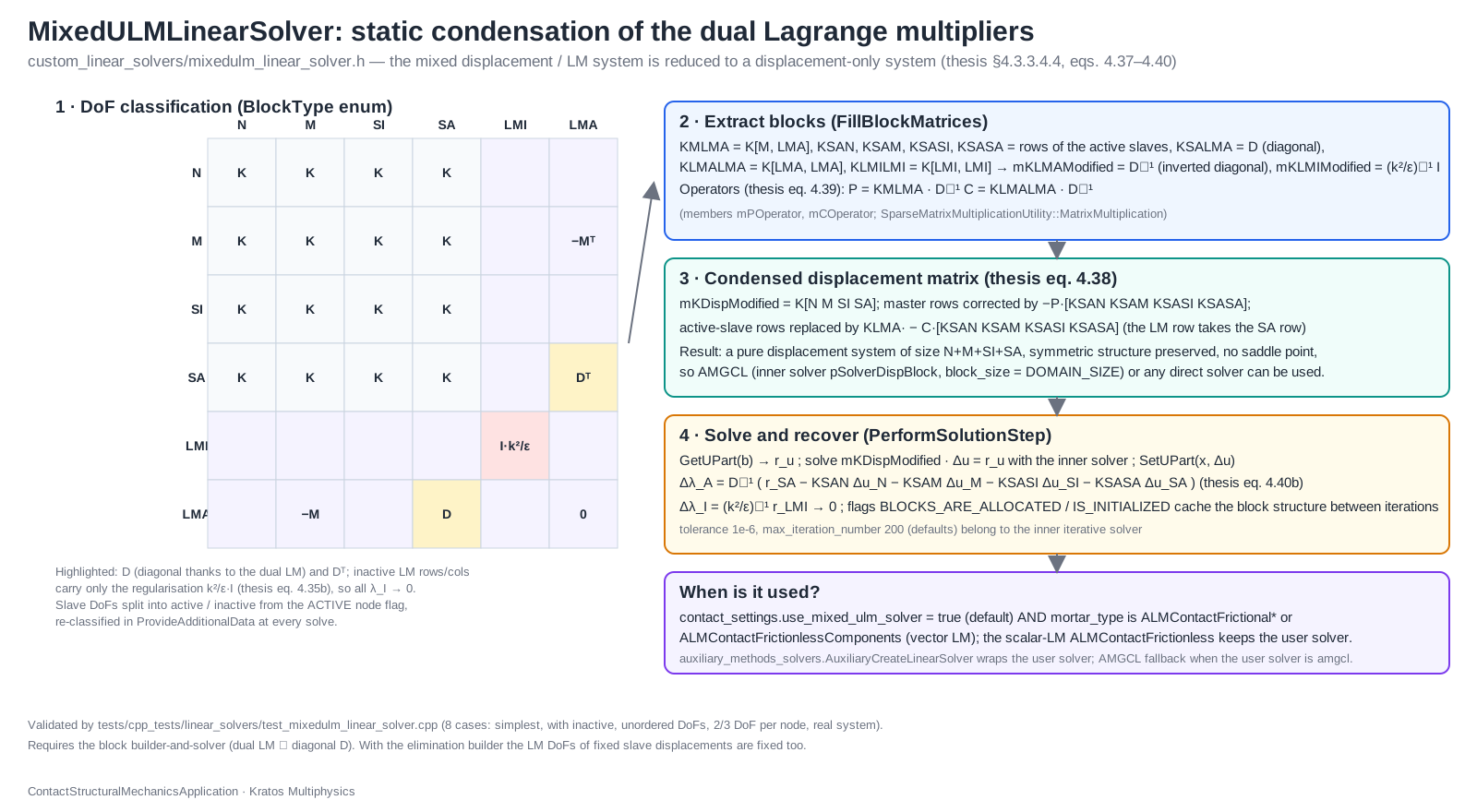
Figure: block classification, sub-block extraction and static condensation performed by the MixedULMLinearSolver (thesis §4.3.3.4.4).
Source. MixedULMLinearSolver<TSparseSpaceType, TDenseSpaceType, TPreconditionerType, TReordererType> derives from IterativeSolver and, in the words of its Doxygen, “is designed for the solution of mixed U-LM problems (this solver in particular is optimized for dual LM, to avoid the resolution)”. It is a wrapper: it owns an inner LinearSolver (mpSolverDispBlock) that solves the condensed displacement system, and performs the condensation and the multiplier recovery itself.
Constructors and defaults
Three constructors are exposed to Python as MixedULMLinearSolver: (LinearSolver), (LinearSolver, double tolerance, size_t max_iteration_number) and (LinearSolver, Parameters). The defaults validated by the last one are
{
    "solver_type"          : "mixed_ulm_linear_solver",
    "tolerance"            : 1.0e-6,
    "max_iteration_number" : 200,
    "echo_level"           : 0
}
tolerance and max_iteration_number are forwarded to the IterativeSolver base and are not used by the condensation itself (the outer problem is solved exactly, the iterations belong to the inner solver). echo_level controls debugging output in Solve: 2 prints the RHS before condensation and the condensed solution and residual, 3 also prints the matrices, 4 or more writes Matrix Market files before_condensation_A_<n>.mm / before_condensation_b_<n>.mm.rhs and A_<n>.mm / b_<n>.mm.rhs (the condensed system) with a running counter mFileCreated. Two local flags track the state: BLOCKS_ARE_ALLOCATED and IS_INITIALIZED.
DoF classification: the BlockType enum
The solver needs to know which row of the system belongs to which kind of DoF, so AdditionalPhysicalDataIsNeeded() returns true and the builder-and-solver calls ProvideAdditionalData(rA, rX, rB, rDofSet, rModelPart) (lines 502-757) before every solve. Every DoF of the set is classified with the flags of its node into
enum class BlockType {
    OTHER,          // any DoF that is not interface displacement or multiplier
    MASTER,         // displacement of an INTERFACE node flagged MASTER
    SLAVE_INACTIVE, // displacement of an INTERFACE SLAVE node that is not ACTIVE
    SLAVE_ACTIVE,   // displacement of an INTERFACE SLAVE node that is ACTIVE
    LM_INACTIVE,    // multiplier (VECTOR_LAGRANGE_MULTIPLIER_X/Y/Z) of a non-ACTIVE node
    LM_ACTIVE       // multiplier of an ACTIVE node
};
The classification fills six index vectors (mOtherIndices, mMasterIndices, mSlaveInactiveIndices, mSlaveActiveIndices, mLMInactiveIndices, mLMActiveIndices), the map mGlobalToLocalIndexing (position of a global row inside its block) and mWhichBlockType. Two consistency checks are enforced with KRATOS_ERROR_IF: the number of classified DoFs must equal rA.size1(), and the number of active multiplier DoFs must equal the number of active slave displacement DoFs (this is what makes \(\mathbf{K}_{S_A\lambda_A}\) square, hence invertible). The block builder-and-solver branch (rModelPart.IsNot(TO_SPLIT)) only counts DoFs with EquationId() < rA.size1(); the elimination branch counts them all. Finally a reordered mDisplacementDofs array (other, master, inactive slave, active slave) is built and handed to the inner solver’s ProvideAdditionalData when it asks for it, so that an AMGCL solver with block_size equal to the space dimension still sees the coordinates in triplets. The solver only classifies the vector multiplier VECTOR_LAGRANGE_MULTIPLIER_X/Y/Z (IsLMDof), which is why it is only used with the components and frictional ALM formulations.
Sub-blocks: FillBlockMatrices
With the ordering \(\mathcal{N}\) (other), \(\mathcal{M}\) (master), \(\mathcal{S}_I\) (inactive slave), \(\mathcal{S}_A\) (active slave), \(\lambda_I\), \(\lambda_A\), the assembled system of a components/frictional ALM problem reads (thesis eq. 4.37, with the block names used in the code comment of FillBlockMatrices)
$$\begin{bmatrix} \mathbf{K}_{NN} & \mathbf{K}_{NM} & \mathbf{K}_{NS_I} & \mathbf{K}_{NS_A} & \mathbf{0} & \mathbf{0} \\ \mathbf{K}_{MN} & \mathbf{K}_{MM} & \mathbf{K}_{MS_I} & \mathbf{K}_{MS_A} & \mathbf{K}_{M\lambda_I} & \mathbf{K}_{M\lambda_A} \\ \mathbf{K}_{S_IN} & \mathbf{K}_{S_IM} & \mathbf{K}_{S_IS_I} & \mathbf{K}_{S_IS_A} & \mathbf{K}_{S_I\lambda_I} & \mathbf{K}_{S_I\lambda_A} \\ \mathbf{K}_{S_AN} & \mathbf{K}_{S_AM} & \mathbf{K}_{S_AS_I} & \mathbf{K}_{S_AS_A} & \mathbf{K}_{S_A\lambda_I} & \mathbf{K}_{S_A\lambda_A} \\ \mathbf{0} & \mathbf{0} & \mathbf{0} & \mathbf{0} & \mathbf{K}_{\lambda_I\lambda_I} & \mathbf{0} \\ \mathbf{0} & \mathbf{K}_{\lambda_AM} & \mathbf{K}_{\lambda_AS_I} & \mathbf{K}_{\lambda_AS_A} & \mathbf{0} & \mathbf{K}_{\lambda_A\lambda_A} \end{bmatrix} \begin{bmatrix} \Delta\mathbf{u}_N \\ \Delta\mathbf{u}_M \\ \Delta\mathbf{u}_{S_I} \\ \Delta\mathbf{u}_{S_A} \\ \Delta\boldsymbol{\lambda}_I \\ \Delta\boldsymbol{\lambda}_A \end{bmatrix} = \begin{bmatrix} \mathbf{r}_N \\ \mathbf{r}_M \\ \mathbf{r}_{S_I} \\ \mathbf{r}_{S_A} \\ \mathbf{r}_{\lambda_I} \\ \mathbf{r}_{\lambda_A} \end{bmatrix}$$
where, in terms of the mortar operators, \(\mathbf{K}_{M\lambda_A} = -k\mathbf{M}_A^T\), \(\mathbf{K}_{S_A\lambda_A} = k\mathbf{D}_{AA}^T\), \(\mathbf{K}_{S_I\lambda_A} = k\mathbf{D}_{IA}^T = \mathbf{0}\) and \(\mathbf{K}_{S_A\lambda_I} = k\mathbf{D}_{AI}^T = \mathbf{0}\) for dual multipliers (the mortar matrix \(\mathbf{D}\) is diagonal, see Mortar integration and dual Lagrange multipliers), \(\mathbf{K}_{\lambda_I\lambda_I} = (k^2/\varepsilon)\mathbf{I}\) is the diagonal that drives the inactive multipliers to zero, and the \(\lambda_A\) row is the linearized weak gap (thesis eqs. 4.36a–4.36b). The first thing FillBlockMatrices (lines 844-1310) does is a parallel CSR pass over rA that counts, and then copies, the entries of every needed sub-block into its own CompressedMatrix:
| Member / local matrix | Block | Rows × columns |
|---|---|---|
KMLMA (local) |
\(\mathbf{K}_{M\lambda_A}\) (the “big block of M”) | master × active LM |
KLMALMA (local) |
\(\mathbf{K}_{\lambda_A\lambda_A}\) | active LM × active LM |
KSALMA (local) |
\(\mathbf{K}_{S_A\lambda_A}\) (the “big block of D”, diagonal) | active slave × active LM |
KLMILMI (local) |
\(\mathbf{K}_{\lambda_I\lambda_I}\) (diagonal) | inactive LM × inactive LM |
mKSAN, mKSAM, mKSASI, mKSASA |
\(\mathbf{K}_{S_AN}\), \(\mathbf{K}_{S_AM}\), \(\mathbf{K}_{S_AS_I}\), \(\mathbf{K}_{S_AS_A}\) | active slave × (other, master, inactive slave, active slave) |
mKLMAModified |
\(\mathbf{K}_{S_A\lambda_A}^{-1}\) | diagonal, computed by ComputeDiagonalByLumping(KSALMA, ...) |
mKLMIModified |
\(\mathbf{K}_{\lambda_I\lambda_I}^{-1}\) | diagonal, ComputeDiagonalByLumping(KLMILMI, ...) |
mPOperator |
\(\mathbf{P} = \mathbf{K}_{M\lambda_A}\,\mathbf{K}_{S_A\lambda_A}^{-1}\) | master × active slave |
mCOperator |
\(\mathbf{C} = \mathbf{K}_{\lambda_A\lambda_A}\,\mathbf{K}_{S_A\lambda_A}^{-1}\) | active LM × active slave |
mKDispModified |
the condensed displacement matrix | (other + master + inactive slave + active slave)² |
ComputeDiagonalByLumping (lines 1936-1985) builds a diagonal matrix with the reciprocal of the diagonal entry rA(i, i) of each row (entries whose absolute value is below ZeroTolerance are left as zero); a row-norm variant is present but commented out. This is exact for the diagonal block produced by dual shape functions and only an approximation if standard multipliers leave off-diagonal entries. The products are computed with SparseMatrixMultiplicationUtility::MatrixMultiplication, and the final matrix is assembled in two passes (ComputeNonZeroColumnsDispDoFs / ComputeAuxiliaryValuesDispDoFs for the rows that are copied, ...PartialDispDoFs for the \(\lambda_A\) rows that replace the \(\mathcal{S}_A\) rows), added with MatrixAdd(mKDispModified, K_disp_modified_aux2, -1.0), symmetrized in structure (EnsureStructuralSymmetryMatrix, so that the sparsity pattern is symmetric even if the values are not) and checked (CheckMatrix). Allocation (AllocateBlocks) happens only the first time or after Clear().
The condensed system
Dropping the zero couplings and imposing \(\Delta\boldsymbol{\lambda}_I = \mathbf{0}\), the multipliers of the active nodes are eliminated with the operators \(\mathbf{P}\) and \(\mathbf{C}\) and the fourth block row is replaced by the constraint row (thesis eq. 4.38):
$$\begin{bmatrix} \mathbf{K}_{NN} & \mathbf{K}_{NM} & \mathbf{K}_{NS_I} & \mathbf{K}_{NS_A} \\ \mathbf{K}_{MN} - \mathbf{P}\mathbf{K}_{S_AN} & \mathbf{K}_{MM} - \mathbf{P}\mathbf{K}_{S_AM} & \mathbf{K}_{MS_I} - \mathbf{P}\mathbf{K}_{S_AS_I} & \mathbf{K}_{MS_A} - \mathbf{P}\mathbf{K}_{S_AS_A} \\ \mathbf{K}_{S_IN} & \mathbf{K}_{S_IM} & \mathbf{K}_{S_IS_I} & \mathbf{K}_{S_IS_A} \\ -\mathbf{C}\mathbf{K}_{S_AN} & \mathbf{K}_{\lambda_AM} - \mathbf{C}\mathbf{K}_{S_AM} & \mathbf{K}_{\lambda_AS_I} - \mathbf{C}\mathbf{K}_{S_AS_I} & \mathbf{K}_{\lambda_AS_A} - \mathbf{C}\mathbf{K}_{S_AS_A} \end{bmatrix} \begin{bmatrix} \Delta\mathbf{u}_N \\ \Delta\mathbf{u}_M \\ \Delta\mathbf{u}_{S_I} \\ \Delta\mathbf{u}_{S_A} \end{bmatrix} = \begin{bmatrix} \mathbf{r}_N \\ \mathbf{r}_M - \mathbf{P}\mathbf{r}_{S_A} \\ \mathbf{r}_{S_I} \\ \mathbf{r}_{\lambda_A} - \mathbf{C}\mathbf{r}_{S_A} \end{bmatrix}$$
with (thesis eq. 4.39, written here with the row/column convention of the code, in which KMLMA is master × LM)
$$\mathbf{P} = \mathbf{K}_{M\lambda_A}\,\mathbf{K}_{S_A\lambda_A}^{-1}, \qquad \mathbf{C} = \mathbf{K}_{\lambda_A\lambda_A}\,\mathbf{K}_{S_A\lambda_A}^{-1}.$$
The thesis writes the combination with a plus sign and \(\mathbf{P} = (\mathbf{K}_{S_A\lambda_A}^{-1}\mathbf{K}_{M\lambda_A})^T\); in the code the sign of the mortar coupling (\(\mathbf{K}_{M\lambda_A} = -k\mathbf{M}_A^T\)) is already inside KMLMA, so the subtraction MatrixAdd(..., -1.0) produces the same matrix. The mechanism is the classic static condensation: because \(\mathbf{K}_{S_A\lambda_A}\) is diagonal, the fourth row of the original system gives \(\Delta\boldsymbol{\lambda}_A\) explicitly in terms of the displacements, and substituting it in the master rows and in the constraint rows removes the multiplier unknowns without any factorization. The resulting matrix is not symmetric (the constraint row replaces the active-slave equilibrium row), but it has no zero diagonal block and its size is the number of displacement DoFs, so algebraic multigrid can be applied to it.
GetUPart (lines 1650-1712) builds the condensed right-hand side exactly as in the formula above (ResidualU of size other + master + inactive slave + active slave, master rows minus mPOperator × r_SA, constraint rows minus mCOperator × r_SA).
PerformSolutionStep: solve, then recover the multipliers
Solve(rA, rX, rB) (lines 416-467) calls Initialize (if not IS_INITIALIZED), InitializeSolutionStep, PerformSolutionStep and FinalizeSolutionStep. InitializeSolutionStep runs FillBlockMatrices (allocating the first time) and initializes the inner solver with mKDispModified; PerformSolutionStep (lines 300-349) then:
- extracts the condensed residual with
GetUPart(rB, mResidualDisp); - solves the displacement block with the inner solver:
mpSolverDispBlock->Solve(mKDispModified, mDisp, mResidualDisp), and scattersmDispback intorX(SetUPart); - recovers the active multipliers from the eliminated equilibrium row of the active slave nodes (thesis eqs. 4.40a–4.40b):
$$\Delta\boldsymbol{\lambda}_A = \mathbf{K}_{S_A\lambda_A}^{-1}\left(\mathbf{r}_{S_A} - \mathbf{K}_{S_AN}\Delta\mathbf{u}_N - \mathbf{K}_{S_AM}\Delta\mathbf{u}_M - \mathbf{K}_{S_AS_I}\Delta\mathbf{u}_{S_I} - \mathbf{K}_{S_AS_A}\Delta\mathbf{u}_{S_A}\right)$$
which is GetLMAPart (the bracket, using mKSAN, mKSAM, mKSASI, mKSASA and the four slices of mDisp) followed by Mult(mKLMAModified, mResidualLMActive, mLMActive) and SetLMAPart;
- recovers the inactive multipliers as \(\Delta\boldsymbol{\lambda}_I = \mathbf{K}_{\lambda_I\lambda_I}^{-1}\mathbf{r}_{\lambda_I}\) (
GetLMIPart,Mult(mKLMIModified, ...),SetLMIPart), which for the ALM residual \(\mathbf{r}_{\lambda_I} = -(k^2/\varepsilon)\boldsymbol{\lambda}_I\) (thesis eq. 4.36b) sets the inactive multipliers to zero, as the thesis prescribes.
Since \(\mathbf{K}_{S_A\lambda_A}\) is diagonal, step 3 is a sparse matrix-vector product and the multiplier recovery is essentially free; the whole cost of the linear solve is the inner solve of step 2. FinalizeSolutionStep and Clear forward to the inner solver and, in the case of Clear, release all blocks and reset the flags. The multi-right-hand-side Solve(rA, DenseMatrix& rX, DenseMatrix& rB) overload returns false without solving (not implemented).
When it is inserted and the AMGCL fallback
auxiliary_methods_solvers.AuxiliaryCreateLinearSolver(main_model_part, settings, contact_settings, linear_solver_settings, linear_solver) (source) is called by _CreateLinearSolver of the contact solvers with the linear solver already created from linear_solver_settings by the structural base class, and decides what the builder-and-solver receives:
- If
contact_settings.rescale_linear_solveristrue, the solver is first wrapped inKM.ScalingSolver(linear_solver, False)(symmetric diagonal scaling of the matrix before the solve; useful because the multiplier rows have a completely different magnitude from the stiffness rows whenMixedULMLinearSolveris not used). - The
MixedULMLinearSolveris considered only whenmortar_typecontainsALMContactFrictionalor equalsALMContactFrictionlessComponents, i.e. when the multiplier is the vectorVECTOR_LAGRANGE_MULTIPLIER; the scalarALMContactFrictionless, the penalty formulations (no multipliers) and mesh tying keep the user’s solver. - In those cases, if
contact_settings.use_mixed_ulm_solveristrue(the default) andcontact_settings.mixed_ulm_solver_parameters.solver_typeismixed_ulm_linear_solver, the log prints “Using MixedULMLinearSolver, definition of ALM parameters recommended” and:- if
linear_solver_settings.solver_typeisamgcl,AMGCLorAMGCLSolver, the user’s AMGCL settings are completed with the following defaults,block_sizeis set toDOMAIN_SIZE, and a newKM.AMGCLSolveris created from them (so that the inner solver works with block matrices of the displacement dimension):
- if
{
    "solver_type"                    : "amgcl",
    "smoother_type"                  : "ilu0",
    "krylov_type"                    : "lgmres",
    "coarsening_type"                : "aggregation",
    "max_iteration"                  : 100,
    "provide_coordinates"            : false,
    "gmres_krylov_space_dimension"   : 100,
    "verbosity"                      : 1,
    "tolerance"                      : 1e-6,
    "scaling"                        : false,
    "block_size"                     : 3,
    "use_block_matrices_if_possible" : true,
    "coarse_enough"                  : 1000,
    "max_levels"                     : -1,
    "post_sweeps"                    : 1,
    "pre_sweeps"                     : 1,
    "preconditioner_type"            : "amg",
    "use_gpgpu"                      : false
}
- for any other
solver_type(a direct solver, for instance) the user’s solver is used as inner solver unchanged; - the returned object is
CSMA.MixedULMLinearSolver(linear_solver, contact_settings["mixed_ulm_solver_parameters"]).- If
mixed_ulm_solver_parameters.solver_typeis anything else, the log prints “Mixed solver not available: … Using not mixed linear solver” and the plain solver is returned; the same happens whenuse_mixed_ulm_solverisfalseor whensettingshas nolinear_solver_settings.
- If
The defaults of contact_settings.mixed_ulm_solver_parameters in AuxiliaryContactSettings are identical to the C++ defaults quoted above. Because the condensation needs the ACTIVE, SLAVE, MASTER and INTERFACE node flags and the vector multiplier DoFs, the solver is not usable outside a contact model part prepared by SearchBaseProcess and the contact solvers (ProvideAdditionalData throws if the DoF count does not match the matrix).
Relation to the thesis
Thesis §4.3.3.4.4 (“Static condensation of the system in considering of the DLMM”) introduces exactly this procedure for the dual Lagrange multiplier method: the global system (eq. 4.37) is partitioned in the six blocks above; since \(\mathbf{K}_{S_I\lambda_A} = \mathbf{0}\), \(\mathbf{K}_{S_A\lambda_I} = \mathbf{0}\) and \(\Delta\boldsymbol{\lambda}_I = \mathbf{0}\), the system is condensed into a pure displacement system (eq. 4.38) with the operators of eq. 4.39, and the active multipliers are recovered a posteriori from the equilibrium of the active slave nodes (eqs. 4.40a–4.40b) “after computing the displacement DoF, from which it depends”. The thesis remarks that the construction “can be applied in any LHS where the LM considered is decomposed in Cartesian components, both frictionless and frictional formulation”, which is precisely the ALMContactFrictionlessComponents / ALMContactFrictional* restriction of the Python wrapper. The diagonality of \(\mathbf{K}_{S_A\lambda_A}\) (“as is the result of the global assemble of the mortar operators D”) is the property that ComputeDiagonalByLumping relies on; with standard (non-dual) multipliers the block is not diagonal and the lumped inverse would only be an approximation, which is one of the reasons why the application uses dual shape functions by default (see Mortar integration and dual Lagrange multipliers).
Tests
tests/cpp_tests/linear_solvers/test_mixedulm_linear_solver.cpp contains eight cases in KratosContactStructuralMechanicsFastSuite, all with a SkylineLUFactorizationSolver as inner solver (an AMGCL alternative is left commented out) and all comparing the MixedULMLinearSolver result with the direct solution of the full mixed system through KRATOS_EXPECT_VECTOR_NEAR:
| Test | System |
|---|---|
MixedULMLinearSolverSimplestSystem |
Minimal hand-built system with one active slave node; also checks the reordered DoF set (EquationId, node id, DISPLACEMENT_X) produced by ProvideAdditionalData |
MixedULMLinearSolverSimplestWithInactiveSystem |
Same with an inactive slave node (exercises the LM_INACTIVE / SLAVE_INACTIVE blocks) |
MixedULMLinearSolverSimplestUnorderedSystem |
Same with the DoFs numbered in a scrambled order (exercises mGlobalToLocalIndexing) |
MixedULMLinearSolverTwoDoFSystem, MixedULMLinearSolverTwoDoFUnorderedSystem |
Two-dimensional nodes, ordered and unordered |
MixedULMLinearSolverThreeDoFSystem, MixedULMLinearSolverThreeDoFUnorderedSystem |
Three-dimensional nodes, ordered and unordered |
MixedULMLinearSolverRealSystem |
A 16 × 16 matrix and its right-hand side extracted from a real 2D contact step, written by CreateAuxiliaryFiles() to A_testing_condensation.mm / b_testing_condensation.rhs, read back with ReadMatrixMarketMatrix / ReadMatrixMarketVector, solved with both solvers and deleted |
The Python tests of the application (ALM_frictional_contact_test_*, ALM_frictionless_components_*, see the Test suite reference) run the solver in its production configuration through AuxiliaryCreateLinearSolver.
A minimal worked example
The first unit test (MixedULMLinearSolverSimplestSystem) is small enough to follow by hand and shows every step of the algorithm. Three nodes carry one DoF each along \(x\): node 1 is an ordinary node, node 2 is an INTERFACE + MASTER node, node 3 is an INTERFACE + SLAVE + ACTIVE node with an additional VECTOR_LAGRANGE_MULTIPLIER_X DoF. The DoF set is \((u_1, u_2, u_3, \lambda_3)\), so ProvideAdditionalData classifies the four rows as OTHER, MASTER, SLAVE_ACTIVE, LM_ACTIVE. The test fills the matrix row by row with \(\sqrt{1}, \sqrt{2}, \dots\) skipping the two entries that couple \(u_1\) with \(\lambda_3\) (an ordinary node never sees a multiplier), and uses \(\mathbf{b} = (1, 2, 3, 4)^T\):
$$\begin{bmatrix} 1 & \sqrt{2} & \sqrt{3} & 0 \\ 2 & \sqrt{5} & \sqrt{6} & \sqrt{7} \\ \sqrt{8} & 3 & \sqrt{10} & \sqrt{11} \\ 0 & \sqrt{12} & \sqrt{13} & \sqrt{14} \end{bmatrix} \begin{bmatrix} \Delta u_1 \\ \Delta u_2 \\ \Delta u_3 \\ \Delta\lambda_3 \end{bmatrix} = \begin{bmatrix} 1 \\ 2 \\ 3 \\ 4 \end{bmatrix}$$
FillBlockMatrices extracts \(\mathbf{K}_{M\lambda_A} = [\sqrt{7}]\), \(\mathbf{K}_{S_A\lambda_A} = [\sqrt{11}]\), \(\mathbf{K}_{\lambda_A\lambda_A} = [\sqrt{14}]\), the active-slave row \(\mathbf{K}_{S_AN} = [\sqrt{8}]\), \(\mathbf{K}_{S_AM} = [3]\), \(\mathbf{K}_{S_AS_A} = [\sqrt{10}]\), computes the scalars \(P = \sqrt{7}/\sqrt{11}\) and \(C = \sqrt{14}/\sqrt{11}\), and assembles the \(3 \times 3\) condensed system in which the third row is the multiplier row \([0, \sqrt{12}, \sqrt{13}]\) corrected by \(C\) times the active-slave row:
$$\begin{bmatrix} 1 & \sqrt{2} & \sqrt{3} \\ 2 - P\sqrt{8} & \sqrt{5} - 3P & \sqrt{6} - P\sqrt{10} \\ -C\sqrt{8} & \sqrt{12} - 3C & \sqrt{13} - C\sqrt{10} \end{bmatrix} \begin{bmatrix} \Delta u_1 \\ \Delta u_2 \\ \Delta u_3 \end{bmatrix} = \begin{bmatrix} 1 \\ 2 - 3P \\ 4 - 3C \end{bmatrix}$$
The inner SkylineLUFactorizationSolver solves this system, and GetLMAPart recovers the multiplier from the eliminated third equation of the original system:
$$\Delta\lambda_3 = \frac{1}{\sqrt{11}}\left(3 - \sqrt{8}\,\Delta u_1 - 3\,\Delta u_2 - \sqrt{10}\,\Delta u_3\right).$$
The test then checks that \((\Delta u_1, \Delta u_2, \Delta u_3, \Delta\lambda_3)\) coincides with the direct solution of the \(4 \times 4\) system to \(10^{-6}\), and that GetDisplacementDofs() returns the three displacement DoFs in the order other, master, active slave with consecutive equation ids. In a real problem \(\mathbf{K}_{S_A\lambda_A}\) is the assembled \(k\mathbf{D}_{AA}^T\) of all the active slave nodes, still diagonal thanks to the dual shape functions, so exactly the same scalar divisions are performed node by node.
Call sequence in one Newton iteration
Putting the two layers together, this is what happens in BuildAndSolve of an ALM components/frictional problem with the default settings (block builder-and-solver, use_mixed_ulm_solver = true, AMGCL inner solver):
ResidualBasedNewtonRaphsonContactStrategy::BaseSolveSolutionStep
└─ ContactResidualBasedBlockBuilderAndSolver::BuildAndSolve
   ├─ Build(...)                              assemble K and b from elements and ComputingContact conditions
   ├─ ApplyDirichletConditions(...)           FixIsolatedNodes → base (rows/cols of fixed DoFs) → FreeIsolatedNodes
   └─ SystemSolveWithPhysics(...)
      ├─ MixedULMLinearSolver::ProvideAdditionalData   classify DoFs (BlockType), build mDisplacementDofs
      │  └─ AMGCLSolver::ProvideAdditionalData          receives the reordered displacement DoFs
      └─ MixedULMLinearSolver::Solve
         ├─ InitializeSolutionStep → FillBlockMatrices  sub-blocks, D⁻¹, P, C, mKDispModified
         ├─ PerformSolutionStep
         │  ├─ GetUPart                                  condensed residual
         │  ├─ AMGCLSolver::Solve(mKDispModified, ...)   displacement increment
         │  ├─ GetLMAPart / Mult(mKLMAModified)           Δλ_A = D⁻¹(r_SA − K_SA· Δu)
         │  └─ GetLMIPart / Mult(mKLMIModified)           Δλ_I = K_λIλI⁻¹ r_λI
         └─ FinalizeSolutionStep
BuildRHS (called before PostCriteria when the RHS must be refreshed, and by the line-search strategy) goes through the same FixIsolatedNodes / FreeIsolatedNodes bracket, so the residual of an isolated multiplier is always zero and cannot pollute the residual-based convergence criteria.
Configuration examples
The default contact configuration needs no explicit choice: with contact_settings.mortar_type = "ALMContactFrictionlessComponents" (or any ALMContactFrictional*) and an AMGCL linear solver, the block builder-and-solver and the condensed solve are selected automatically.
"solver_settings" : {
    "solver_type"                : "Static",
    "builder_and_solver_settings" : {
        "type" : "block"
    },
    "linear_solver_settings"     : {
        "solver_type" : "amgcl"
    },
    "contact_settings"           : {
        "mortar_type"           : "ALMContactFrictionlessComponents",
        "use_mixed_ulm_solver"  : true,
        "rescale_linear_solver" : false,
        "mixed_ulm_solver_parameters" : {
            "solver_type"          : "mixed_ulm_linear_solver",
            "tolerance"            : 1.0e-6,
            "max_iteration_number" : 200,
            "echo_level"           : 0
        }
    }
}
To solve the full saddle-point system with a direct solver instead (for small problems, or to compare with the condensed solution), disable the wrapper:
"linear_solver_settings" : {
    "solver_type" : "skyline_lu_factorization"
},
"contact_settings" : {
    "mortar_type"          : "ALMContactFrictional",
    "use_mixed_ulm_solver" : false
}
To use the elimination builder-and-solvers (fixed slave displacements that must fix the corresponding multipliers, or constraints acting on interface nodes):
"builder_and_solver_settings" : {
    "type" : "elimination"
},
"multi_point_constraints_used" : true,
"contact_settings" : {
    "mortar_type" : "ALMContactFrictionlessComponents"
}
With this last configuration ContactResidualBasedEliminationBuilderAndSolverWithConstraints is created, the computing model part is flagged TO_SPLIT if constraints exist, and MixedULMLinearSolver::ProvideAdditionalData takes its elimination branch.
mortar_type |
Multiplier DoFs | System handed to the linear solver (default settings) |
|---|---|---|
ALMContactFrictionless |
LAGRANGE_MULTIPLIER_CONTACT_PRESSURE (scalar) |
Full mixed system (no condensation; the scalar multiplier is not classified by IsLMDof) |
ALMContactFrictionlessComponents |
VECTOR_LAGRANGE_MULTIPLIER |
Condensed displacement system through MixedULMLinearSolver |
ALMContactFrictional, ALMContactFrictionalPureSlip |
VECTOR_LAGRANGE_MULTIPLIER |
Condensed displacement system through MixedULMLinearSolver |
PenaltyContactFrictionless, PenaltyContactFrictional* |
none | Displacement system as assembled |
ScalarMeshTying, ComponentsMeshTying |
SCALAR_LAGRANGE_MULTIPLIER / VECTOR_LAGRANGE_MULTIPLIER |
Full mixed system (mesh tying is not routed through the wrapper) |
Practical notes
- With
builder_and_solver_settings.type = "block"and a scalar ALM (ALMContactFrictionless) the full saddle-point system reaches the linear solver; a direct solver oramgclwith a suitable smoother is needed. Switching toALMContactFrictionlessComponentsenables the condensation at the price of \(d\) multipliers per node instead of one. rescale_linear_solveranduse_mixed_ulm_solvercan be combined: the scaling wrapper is applied to the inner solver, that is to the condensed displacement system.- The elimination builder-and-solvers are the ones to use when slave nodes have prescribed displacements in the direction of the contact normal (symmetry planes crossing the interface); with the block builder-and-solver the corresponding multiplier is left free and the interface may not converge.
echo_level >= 4inmixed_ulm_solver_parametersis the easiest way to export the matrices before and after condensation for offline analysis.